The Hybrid equivalent model

The hybrid equivalent model is a linearized representation of a nonlinear device, allowing engineers to predict circuit behavior with manageable calculations. A hybrid equivalent model is a modeling approach in electronics and circuit theory for representing systems that combine active and passive components. It's particularly useful for analyzing transistors and other nonlinear devices, where direct mathematical treatment can be complex. The hybrid model replaces the actual device with a simplified circuit containing controlled sources and resistances, making analysis easier. The parameters of the hybrid equivalent circuit are defined in general terms for any operating conditions. In other words, the hybrid parameters may not reflect the actual operating conditions but simply indicate the expected levels of each parameter for general use. Because all specification sheets provide the hybrid parameters, the model is still extensively used.

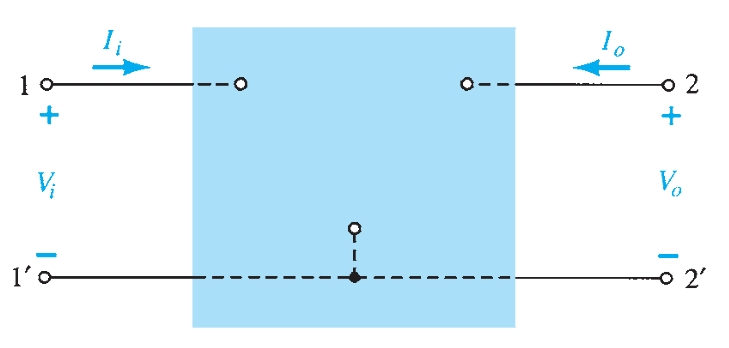
The description of the hybrid equivalent model will begin with the general two-port system. The following set of equations is only one of a number of ways in which the four variables of a 2-port system can be related.

\[V_{i} = h_{11}I_{i} + h_{12}V_{o}\]

\[I_{o} = h_{21}I_{i} + h_{22}V_{o}\]

\[\begin{bmatrix} V_{i} \\ I_{o}\\ \end{bmatrix} = \begin{bmatrix} h_{11} & h_{12} \\ h_{21} & h_{22}\\ \end{bmatrix} \begin{bmatrix} I_{i} \\ V_{o}\\ \end{bmatrix} \]

The parameters relating the four variables are called h-parameters, from the word ``hybrid." The term hybrid was chosen because the mixture of variables (\((V\, \text{and}\, I)\) in each equation results in a hybrid set of units of measurement for the h-parameters.

Finding \(h_{11}\): Set \(V_{o} = 0\) (short circuit the output terminals) and solve for \(h_{11}\). \[h_{11} = \frac{V_{i}}{I_{i}}\bigg|_{V_{o}=0} \quad \text{ohms}\] The ratio indicates that the parameter \(h_{11}\) is an impedance parameter with the units of ohms. Because it is the ratio of the input voltage to the input current with the output terminals shorted, it is called the short-circuit input impedance parameter. The subscript \(11\) of \(h_{11}\) refers to the fact that the parameter is determined by a ratio of quantities measured at the input terminals.
Finding \(h_{12}\): Set \(I_{i} = 0\) by opening the input leads, the following results for \(h_{12}\). \[h_{12} = \frac{V_{i}}{V_{o}}\bigg|_{I_{i}=0} \quad \text{unitless}\] The parameter \(h_{12}\), therefore, is the ratio of the input voltage to the output voltage with the input current equal to zero. It has no units because it is a ratio of voltage levels and is called the open-circuit reverse transfer voltage ratio parameter. The subscript \(12\) of \(h_{12}\) indicates that the parameter is a transfer quantity determined by a ratio of input \((1)\) to output \((2)\) measurements. The first integer of the subscript defines the measured quantity to appear in the numerator; the second integer defines the source of the quantity to appear in the denominator. The term reverse is included because the ratio is an input voltage over an output voltage
Finding \(h_{21}\): Setting \(V_{o}\) is set equal to zero by again shorting the output terminals, the following results for \(h_{21}\) : \[h_{21} = \frac{I_{o}}{I_{i}}\bigg|_{V_{o}=0} \quad \text{unitless}\] the ratio of an output quantity to an input quantity. The term forward
will now be used rather than reverse as indicated for \(h_{12}\). The parameter \(h_{21}\) is the ratio of the output current to the input current with the output terminals shorted. This parameter, like \(h_{12}\), has no units because it is the ratio of current levels. It is formally called the short-circuit forward transfer current ratio parameter. The subscript \(21\) again indicates that it is a transfer parameter with the output quantity \((2)\) in the numerator and the input quantity \((1)\) in the denominator.
Finding \(h_{22}\) : The last parameter, \(h_{22}\), can be found by again opening the input leads to set \(I_{1} = 0\) and solving for \(h_{22}\) \[h_{22} = \frac{I_{o}}{V_{o}}\bigg|_{I_{i}=0} \quad \text{siemens}\] Because it is the ratio of the output current to the output voltage, it is the output conductance parameter, measured in siemens \((S)\). It is called the open-circuit output admittance parameter. The subscript \(22\) indicates that it is determined by a ratio of output quantities.

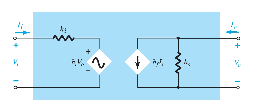
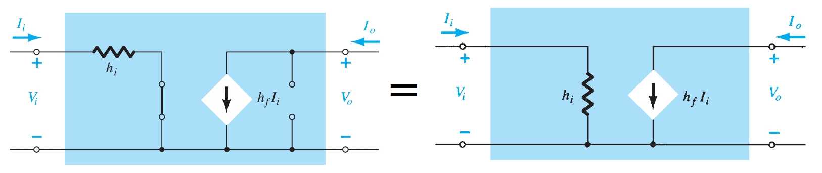
The complete ``\(ac\)" equivalent circuit for the basic three-terminal linear device with a new set of subscripts for the h-parameters. The notation is of a more practical nature because it relates the \(h\)-parameters to the resulting ratio obtained in the last few paragraphs. The choice of letters is obvious from the following listing:

\(h_{11}\) \(\Rightarrow\) input resistance \(\Rightarrow\) \(h_{i}\)
\(h_{12}\) \(\Rightarrow\) reverse transfer voltage ratio \(\Rightarrow\) \(h_{r}\)
\(h_{21}\) \(\Rightarrow\) forward transfer current ratio \(\Rightarrow\) \(h_{f}\)
\(h_{22}\) \(\Rightarrow\) output conductance \(\Rightarrow\) \(h_{o}\)

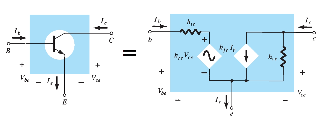
The \(h\)-parameters will change with each configuration. To distinguish which parameter has been used or which is available, a second subscript has been added to the \(h\)-parameter notation. For the common-base configuration, the lowercase letter \(b\) was added, whereas for the common-emitter and common-collector configurations, the letters \(e\) and \(c\) were added, respectively. The hybrid equivalent network for the common-emitter configuration is shown in standard notation. \(I_{i} = I_{b}\), \(I_{o} = I_{c}\), and, through an application of Kirchhoff’s current law, \(I_{e} = I_{b} + I_{c}\).

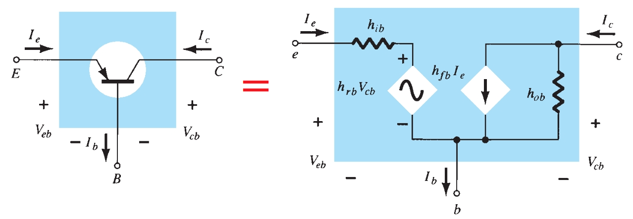
The input voltage is now \(V_{be}\), with the output voltage \(V_{ce}\). For the common-base configuration, \(I_{i} = I_{e}\), \(I_{o} = I_{c}\) with \(V_{eb} = V_{i}\) and \(V_{cb} = V_{o}\).

For the common-emitter and common-base configurations, the magnitude of \(h_{r}\) and \(h_{o}\) is often such that the results obtained for the important parameters such as \(Z_{i}\), \(Z_{o}\), \(A_{v}\), and \(A_{i}\) are only slightly affected if \(h_{r}\) and \(h_{o}\) are not included in the model. Because \(h_{r}\) is normally a relatively small quantity, its removal is approximated by \(h_{r} = 0\) and \(h_{r}V_{o} = 0\), resulting in a short-circuit equivalent for the feedback element. The resistance determined by \(\frac{1}{h_{o}}\) is often large enough to be ignored in comparison to a parallel load, permitting its replacement by an open-circuit equivalent for the \(CE\) and \(CB\) models.

The resulting equivalent is quite similar to the general structure of the common-base and common-emitter equivalent circuits obtained with the \(r_{e}\) model.

In fact, the hybrid equivalent and the \(r_{e}\) models.

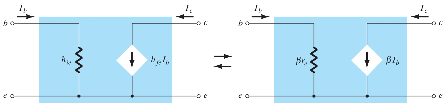
For CE configuration:

Figure .

\[h_{ie}=\beta\,r_{e}\]
and
\[h_{fe}=\beta_{ac}\]
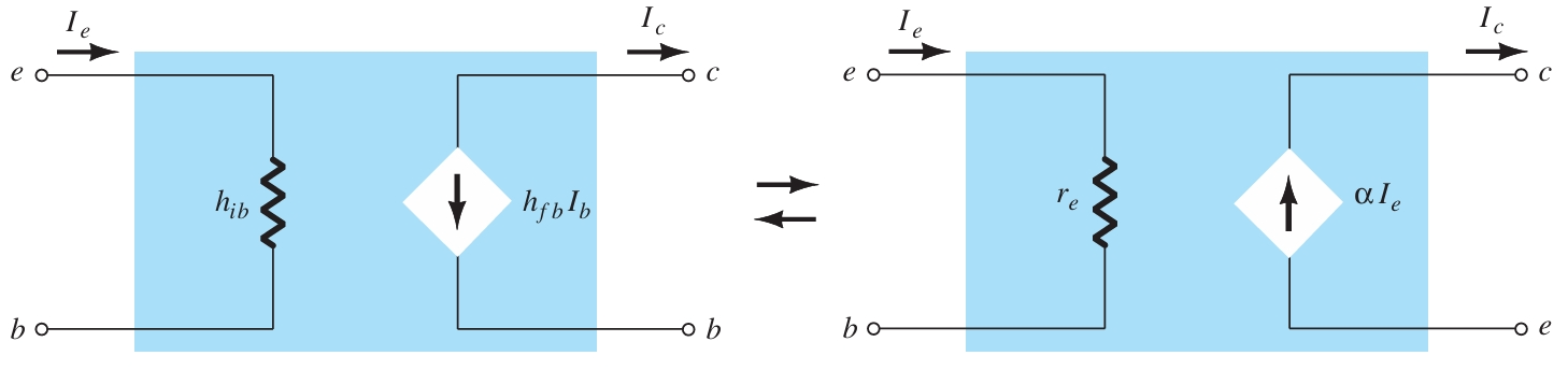
For CB configuration,

Figure .

\[h_{ib}=r_{e} \]
and
\[h_{fb}=-\alpha = -1 \]

The minus sign accounts for the fact that the current source of the standard hybrid equivalent circuit is pointing down rather than in the actual direction as shown in the \(r_{e}\) model.

A series of equations relating the parameters of each configuration for the hybrid equivalent circuit. The hybrid parameter \(h_{fe} (\beta_{ac})\) is the least sensitive of the hybrid parameters to a change in collector current. Assuming, therefore, that \(h_{fe} = beta\) is a constant for the range of interest, is a fairly good approximation. It is \(h_{ie} = \beta\,r_{e}\) that will vary significantly with \(I_{C}\) and should be determined at operating levels because it can have a real effect on the gain levels of a transistor amplifier.