Feedback Concept
Feedback is a concept of feeding back a fraction of output (Voltage/Current) to the input. Depending on the relative polarity of the signal being fed back into a circuit, one may have negative or positive feedback.
- Negative feedback results in decreased voltage gain, for which a number of circuit features are improved.
- Positive feedback drives a circuit into oscillation as in various types of oscillator circuits.
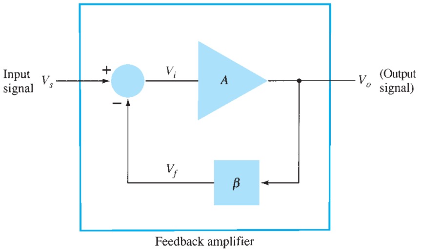
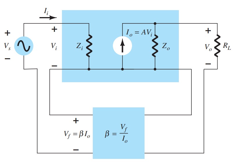
A typical feedback connection is shown in Fig 1. The input signal \(V_{s}\) is applied to a mixer network, where it is combined with a feedback signal \(V_{f}\). The difference of these signals \(V_{i}\) is then the input voltage to the amplifier. A portion of the amplifier output \(V_{o}\) is connected to the feedback network (\(\beta\)), which provides a reduced portion of the output as a feedback signal to the input mixer network.
If the feedback signal is of the opposite polarity to the input signal, negative feedback results. Although negative feedback results in reduced overall voltage gain, several improvements are obtained, among them being:
- Higher input impedance.
- Better stabilized voltage gain.
- Improved frequency response.
- Lower output impedance.
- Reduced noise.
- More linear operation.
Types of Feedback Connection
There are four basic ways of connecting the feedback signal. Both voltage and current can be fed back to the input either in series or parallel. Specifically, there can be:
- Voltage-series feedback
- Voltage-shunt feedback
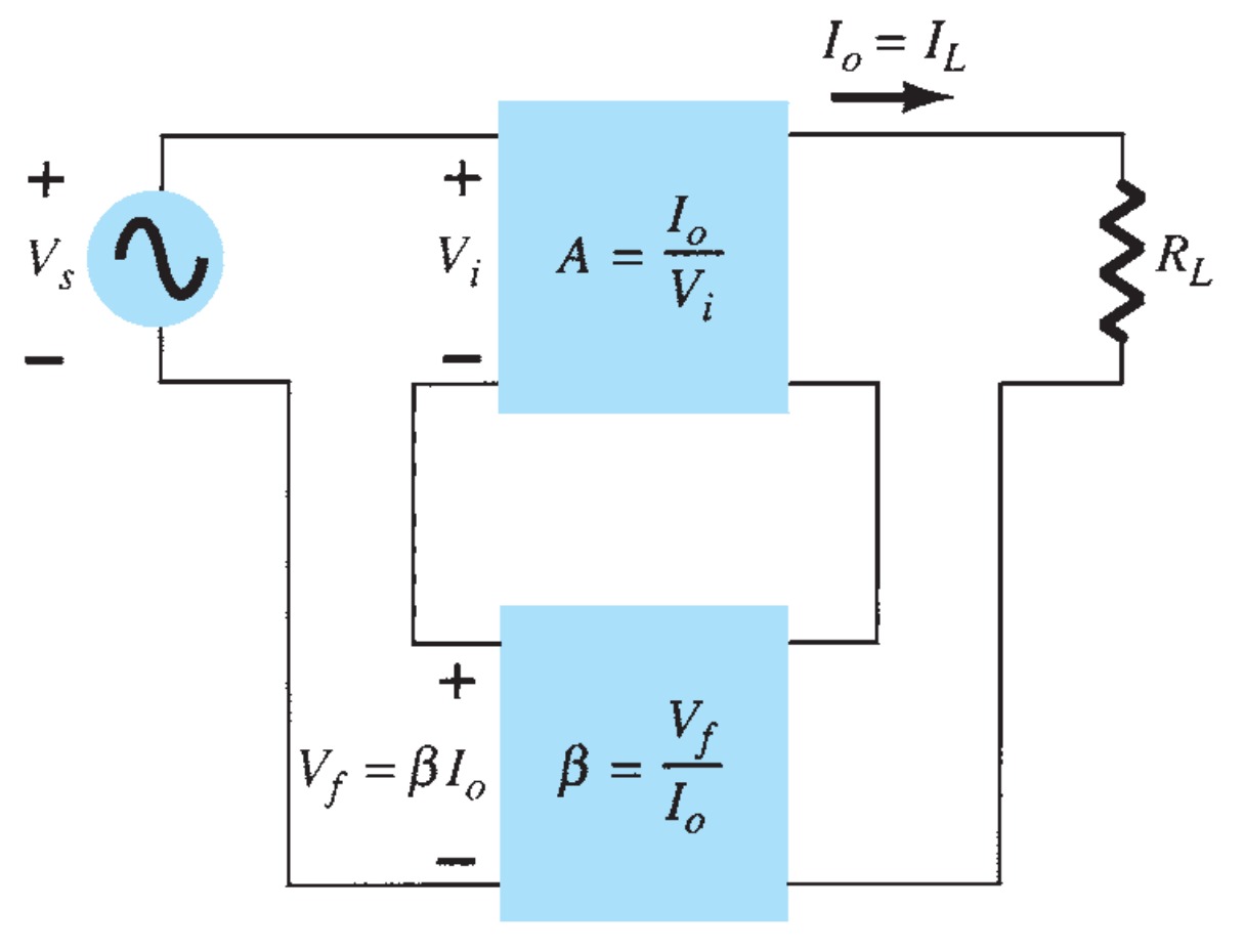
- Current-series feedback
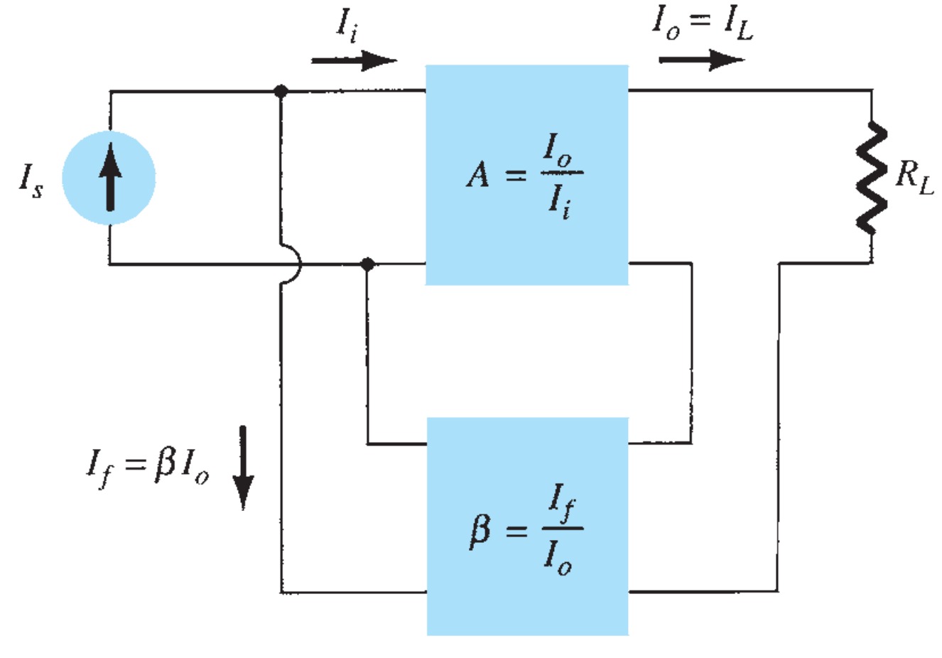
- Current-shunt feedback
In the above list,
- Voltage refers to connecting the output voltage as input to the feedback network;
- Current refers to tapping off some output current through the feedback network.
- Series refers to connecting the feedback signal in series with the input signal voltage;
- Shunt refers to connecting the feedback signal in shunt (parallel) with an input current source.
- Series feedback connections tend to increase the input resistance
- Shunt feedback connections tend to decrease the input resistance.
- Voltage feedback tends to decrease the output impedance
- Current feedback tends to increase the output impedance.
Typically, higher input and lower output impedances are desired for most cascade amplifiers. Both of these are provided using the voltage-series feedback connection.
The gain without feedback, \(A\), is that of the amplifier stage. With feedback \(\beta\), the overall gain of the circuit is reduced by a factor \((1 + \beta A)\). A summary of the gain, feedback factor, and gain with feedback is provided for reference in Table 1.
| Voltage-Series | Voltage-Shunt | Current-Series | Current-Shunt | |
|---|---|---|---|---|
| Gain without feedback (\(A\)) | \(\frac{V_{o}}{V_{i}}\) | \(\frac{V_{o}}{I_{i}}\) | \(\frac{I_{o}}{V_{i}}\) | \(\frac{I_{o}}{I_{i}}\) |
| Feedback (\(\beta\)) | \(\frac{V_{f}}{V_{o}}\) | \(\frac{I_{f}}{V_{o}}\) | \(\frac{V_{f}}{I_{o}}\) | \(\frac{I_{f}}{I_{o}}\) |
| Gain with feedback (\(A_{f}\)) | \(\frac{V_{o}}{V_{s}}\) | \(\frac{V_{o}}{I_{s}}\) | \(\frac{I_{o}}{V_{s}}\) | \(\frac{I_{o}}{I_{s}}\) |
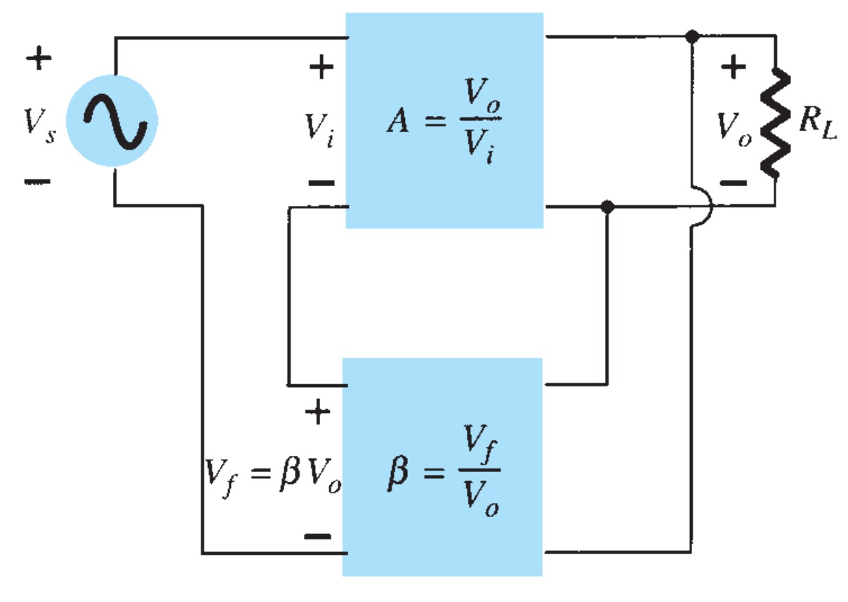
Voltage-Series Feedback
Figure 3 shows the voltage-series feedback connection with a part of the output voltage fed back in series with the input signal, resulting in an overall gain reduction. If there is no feedback (\(V_{f} = 0\)), the voltage gain of the amplifier stage is
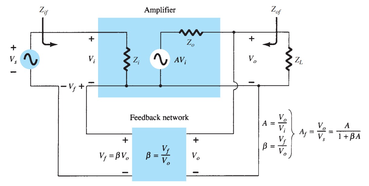
\[A = \frac{V_{o}}{V_{s}} = \frac{V_{o}}{V_{i}}\]
If a feedback signal \(V_{f}\) is connected in series with the input, then \[ V_{i} = V_{s} - V_{f}\] Since \[V_{o} = AV_{i} = A(V_{s} - V_{f}) = AV_{s} - AV_{f} = AV_{s} - A(\beta V_{o}) \] then \[(1 + \beta A)V_{o} = AV_{s}\] so that the overall voltage gain with feedback is \[ A_{f} = \frac{V_{o}}{V_{s}} = \frac{A}{1 + \beta A} \]
Equation shows that the gain with feedback is the amplifier gain reduced by the factor (\(1 + \beta A\) ). This factor will be seen also to affect input and output impedance among other circuit features.
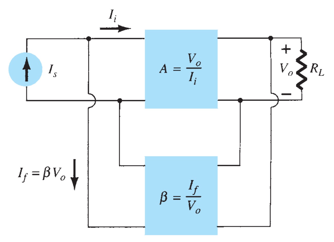
Voltage-Shunt Feedback
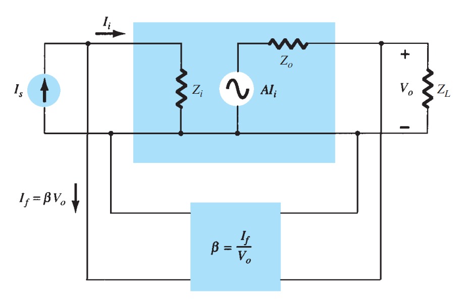
The gain with feedback for the network of Fig 4. is
\[A_{f} = \frac{V_{o}}{I_{s}} = \frac{A I_{i}}{I_{i} + I_{f}} = \frac{A I_{i}}{I_{i} + \beta V_{o}} = \frac{A I_{i}}{I_{i} + \beta A I_{i}}\] \[ A_{f} = \frac{A}{1 + \beta A}\]
Input Impedance with Feedback
Voltage-Series Feedback
A more detailed voltage-series feedback connection is shown in Fig 4. The input impedance can be determined as follows: \[I_{i} = \frac{V_{i}}{Z_{i}} = \frac{V_{s} - V_{f}}{Z_{i}} = \frac{V_{s} - \beta V_{o}}{Z_{i}} = \frac{V_{s} - \beta AV_{i}}{Z_{i}}\] \[I_{i} Z_{i} = V_{s} - \beta AV_{i}\] \[V_{s} = I_{i}Z_{i} + \beta AV_{i} = I_{i}Z_{i} + \beta AI_{i}Z_{i}\] \[ Z_{if} = \frac{V_{s}}{I_{i}} = Z_{i} + (\beta A)Z_{i} = Z_{i}(1 + \beta A)\]
The input impedance with series feedback is seen to be the value of the input impedance without feedback multiplied by the factor (\(1 + \beta A \)), and applies to both voltage-series and current-series configurations.
Voltage-Shunt Feedback
A more detailed voltage-shunt feedback connection is shown in Fig 4. The input impedance can be determined to be
\[Z_{if} = \frac{V_{i}}{I_{s}} = \frac{V_i}{I_{i} + I_{f}} = \frac{V_{i}} {I_{i} + \beta V_{o}}\] \[ = \frac{\frac{V_{i}}{I_{i}}} {\frac{I_{i}}{I_{i}} + \frac{\beta V_{o}}{I_{i}}}\] \[ Z_{if} = \frac{Z_{i}}{1 + \beta A}\]
This reduced input impedance applies to the voltage-series connection of Fig 3. and the voltage-shunt connection of Fig 4.
Output Impedance with Feedback
The output impedance for the connections of Fig 3 and 4. is dependent on whether voltage or current feedback is used. For voltage feedback, the output impedance is decreased, whereas current feedback increases the output impedance.
Voltage-Series Feedback
The voltage-series feedback circuit of Fig 3. provides sufficient circuit detail to determine the output impedance with feedback. The output impedance is determined by applying a voltage \(V_{o}\), resulting in a current \(I_{o}\), with \(V_{s}\) shorted out \(V_s = 0)\). The voltage \(V_{i}\)s then
\[ V_{o} = I_{o}Z_{o} + AV_{i}\] For \[V_{s} = 0, V_{i} = -V_{f}\] so that \[V_{o} = I_{o}Z_{o} - AV_{f} = I_{o}Z_{o} - A(\beta V_{o})\] Rewriting the equation as \[V_{o} + \beta AV_{o} = I_{o}Z_{o}\] allows solving for the output impedance with feedback: \[Z_{of} = \frac{V_{o}}{I_{o}} = \frac{Z_{o}}{1 + \beta A}\]
Current-Series Feedback
The output impedance with current-series feedback can be determined by applying a signal \(V\) to the output with \(V_{s}\) shorted out, resulting in a current \(I\), the ratio of \(V\) to \(I\) being the output impedance. Figure 5 shows a more detailed connection with current-series feedback.
Current-series feedback connection.
For the output part of a current-series feedback connection, the resulting output impedance is determined as follows.
With \(V_{s}\) = 0,
\[ V_{i} = V_{f}\] \[I = \frac{V}{Z_{o}}- AV_{i} = \frac{V}{Z_{o}}- AV_{f} = \frac{V}{Z_{o}}- A\beta I \] \[Z_{o}(1 + \beta A)I = V\] \[Z_{of} = \frac{V}{I} = Z_{o}(1 + \beta A)\]
A summary of the effect of feedback on input and output impedance is provided in Table.
Effect of Feedback Connection on Input and Output Impedance
| Voltage-Series | Current-Series | Voltage-Shunt | Current-Shunt |
|---|---|---|---|
| \(Z_{if} = Z_{i}(1 + \beta A)\) | \(\frac{Z_{i}}{(1 + \beta A)}\) | \(\frac{Z_{i}}{1 + \beta A}\) | \(\frac{Z_{i}}{1 + \beta A}\) |
| (increased) | (increased) | decreased) | (decreased) |
| \(Z_{of} = \frac{Z_{o}}{1 + \beta A}\) | \(Z_{o}(1 + \beta A)\) | \(\frac{Z_{o}}{1 + \beta A}\) | \(Z_{o}(1 + \beta A)\) |
| (decreased) | (increased) | decreased) | (increased) |
Advantages of Negative feedback
Reduction in Frequency Distortion
For a negative-feedback amplifier having \(\beta A\) \(\gt\gt \,1\), the gain with feedback is \(A_{f} \sim 1/\beta\). It follows from this that if the feedback network is purely resistive, the gain with feedback is not dependent on frequency even though the basic amplifier gain is frequency dependent. Practically, the frequency distortion arising because of varying amplifier gain with frequency is considerably reduced in a negative-voltage feedback amplifier circuit.
Reduction in Noise and Nonlinear Distortion
Signal feedback tends to hold down the amount of noise signal (such as power-supply hum) and nonlinear distortion. The factor \((1 + \beta A)\) reduces both input noise and resulting nonlinear distortion for considerable improvement. However, there is a reduction in overall gain (the price required for the improvement in circuit performance). If additional stages are used to bring the overall gain up to the level without feedback, the extra stage(s) might introduce as much noise back into the system as that reduced by the feedback amplifier. This problem can be somewhat alleviated by readjusting the gain of the feedback amplifier circuit to obtain higher gain while also providing reduced noise signal.
Effect of Negative Feedback on Gain and Bandwidth
The overall gain with negative feedback is shown to be
\[A_{f} = \frac{A}{1 + \beta A} = \frac{A}{\beta A} = \frac{1}{\beta}\] \[\text{for}\, \quad \beta A \gt\gt 1\]
As long as \(\beta A \gt\gt 1\), the overall gain is approximately \(1/\beta\). For a practical amplifier (for single low- and high-frequency breakpoints) the open-loop gain drops off at high frequencies due to the active device and circuit capacitances. Gain may also drop off at low frequencies for capacitively coupled amplifier stages. Once the open-loop gain \(A\) drops low enough and the factor \(\beta A\) is no longer much larger than \(1\), the conclusion of Eq. that \(A_{f} \sim 1/\beta\) no longer holds true.
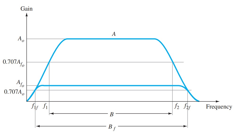
Figure 6 shows that the amplifier with negative feedback has more bandwidth (\(B_{f}\)) than the amplifier without feedback (\(B\)). The feedback amplifier has a higher upper \(3\, \text{dB}\) frequency and smaller lower \(3\, \text{dB}\) frequency
Gain Stability with Feedback
In addition to the \(\beta\) factor setting a precise gain value, we are also interested in how stable the feedback amplifier is compared to an amplifier without feedback.
Differentiating feedback gain Eq. leads to
\[\frac{dA_{f}}{A_{f}} = \frac{1}{1 + \beta A}\frac{dA}{A} \]
\[\frac{dA_{f}}{A_{f}} = \frac{1}{\beta A}\frac{dA}{A} \] \[\text{for}\, \beta A \gt\gt 1\]
This shows that magnitude of the relative change in gain \(\frac{dA_{f}}{A_{f}}\) is reduced by the factor \(\beta A\) compared to that without feedback \(\frac{dA}{A}\).
Practical Feedback Circuits
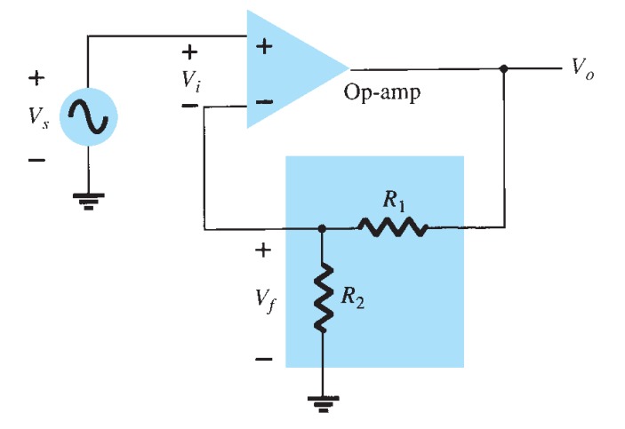
Voltage-Seris Feedback
Figure 7 shows a voltage-series feedback connection using an op-amp. The gain of the op-amp, \(A\), without feedback, is reduced by the feedback factor \[\beta = \frac{R_2}{R_1 + R_2}\]
Voltage-Shunt Feedback
The constant-gain op-amp circuit of Figure 8. a provides voltage-shunt feedback. Referring to Figure 8 and Table 1 and the op-amp ideal characteristics \(I_i = 0\), \(V_i = 0\), and voltage gain of infinity, we have
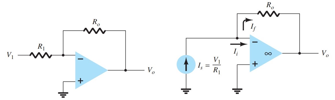
\[A = \frac{V_{o}}{I_{i}} = \infty \] \[\beta = \frac{I_{f}}{V_{o}} = = \frac{-1}{R_{o}}\]
The gain with feedback is then \[A_{f} = \frac{V_{o}}{I_{s}} = \frac{V_{o}}{I_{i}} = \frac{A}{1 + \beta A} = \frac{1}{\beta} = -R_{o}\] This is a transfer resistance gain. The more usual gain is the voltage gain with feedback, \[ A_{vf} = \frac{V_{o}}{I_{s}} \frac{I_{s}}{V_{1}} = (-R_{o})\frac{1}{R_{1}} = \frac{-R_{o}}{R_{1}}\]
Nyquist Criterion
In judging the stability of a feedback amplifier as a function of frequency, the \(\beta A\) product and the phase shift between input and output are the determining factors. One of the most popular techniques used to investigate stability is the Nyquist method. A Nyquist diagram is used to plot gain and phase shift as a function of frequency on a complex plane. The Nyquist plot, in effect, combines the two Bode plots of gain versus frequency and phase shift versus frequency on a single plot. A Nyquist plot is used to quickly show whether an amplifier is stable for all frequencies and how stable the amplifier is relative to some gain or phase-shift criteria.
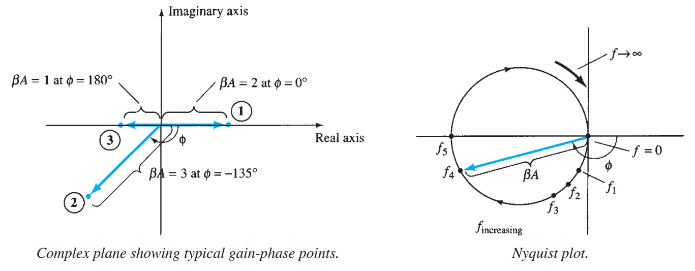
As a start, consider the complex plane shown in Fig 9. A few points of various gain \((\beta A)\) values are shown at a few different phase-shift angles. By using the positive real axis as reference \((0°)\), we see a magnitude of \(\beta A = 2\) at a phase shift of \((0°)\) at point \((1)\). Additionally, a magnitude of \(\beta A = 3\) at a phase shift of \((-135°)\) is shown at point \(2\) and a magnitude/phase of \(\beta A = 1\) at \(180°\) is shown at point \(3\). Thus points on this plot can represent both gain magnitude of \(\beta A\) and phase shift.
If the points representing gain and phase shift for an amplifier circuit are plotted at increasing frequency, then a Nyquist plot is obtained as shown by the plot in Fig 9. At the origin, the gain is \(0\) at a frequency of \(0\) (for \(RC\) -type coupling). At increasing frequency, points \(f_1\), \(f_2\), and \(f_3\) and the phase shift increase, as does the magnitude of \(\beta A\) . At a representative frequency \(f_4 \), the value of \(A\) is the vector length from the origin to point \(f_4\) and the phase shift is the angle \(f\). At a frequency \(f_5\), the phase shift is \(180°\). At higher frequencies, the gain is shown to decrease back to \(0\).
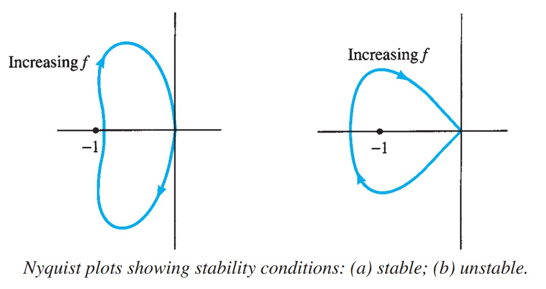
The Nyquist criterion for stability can be stated as follows:
The amplifier is unstable if the Nyquist curve encloses (encircles) the \(-1\) point, and it is stable otherwise.
An example of the Nyquist criterion is demonstrated by the curves in Fig 20. The Nyquist plot in Fig 10. a is stable since it does not encircle the \(-1\) point, whereas that shown in Fig 10. is unstable since the curve does encircle the \(-1\) point. Keep in mind that encircling the \(-1\) point means that at a phase shift of \(180°\) the loop gain \(\beta A \) is greater than \(1\); therefore, the feedback signal is in phase with the input and large enough to result in a larger input signal than that applied, with the result that oscillation occur.
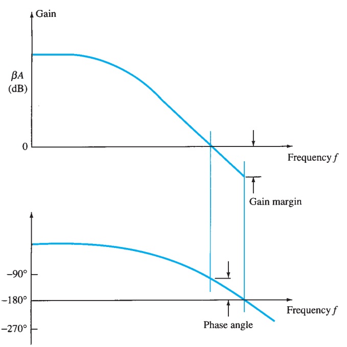
Gain and Phase Margins
From the Nyquist criterion, we know that a feedback amplifier is stable if the loop gain (\(\beta A\) ) is less than unity (\(0 \,\text{dB}\)) when its phase angle is \(180°\). We can additionally determine some margins of stability to indicate how close to instability the amplifier is. That is, if the gain \((\beta A)\) is less than unity but, say, \(0.95\) in value, this would not be as relatively stable as another amplifier having, say, \(\beta A = 0.7\) (both measured at \(180°\)). Of course, amplifiers with loop gains \(0.95\) and \(0.7\) are both stable, but one is closer to instability, if the loop gain increases, than the other.
We can define the following terms:
\(\text{Gain margin (GM)}\) is defined as the negative of the value of \(\beta A\) in decibels at the frequency at which the phase angle is \(180°\). Thus, \(0 \,\text{dB}\), equal to a value of \(\beta A = 1\), is on the border of stability and any negative decibel value is stable. The GM may be evaluated in decibels from the curve of Fig 11.
\(\text{Phase margin (PM)}\) is defined as the angle of \(180°\) minus the magnitude of the angle at which the value \(\beta A\) is unity (\(0 \,\text{dB}\)). The \(PM\) may also be evaluated directly from the curve of Fig 11.