Analog Computing
Operational amplifiers (op-amps) are versatile analog devices that can be configured to perform mathematical operations such as addition, subtraction, integration, and differentiation. By combining these functions, it is possible to design circuits that solve ordinary differential equations (ODEs) in real time. This approach is widely used in analog computers, control systems, and signal processing, making op-amps powerful tools in analog computation and system modeling. Solving differential equations with op-amps involves translating mathematical operations into circuit equivalents. Differentiators, integrators, summing amplifiers, and gain stages form the building blocks. By carefully designing the circuit, the real-time solutions to ODEs can be obtained.
The OP-AMP circuit can be designed following the steps given.
- The first step is to write the given equation in its standard mathematical form.
- Each term in the equation corresponds to a mathematical operation, namely, summation, differentiation, integration, multiplication, and subtraction.
- Map the mathematical operation to the respective OP-AMP circuit and calculate the values of the passive components as required to get the appropriate outputs for each of the OP-AMP circuits.
- Then construct the block diagram to generate the desired output voltage for the differential equation. This block diagram ensures that the circuit output corresponds to its solution.
Method
Consider a differential equation:
\[\frac{dy}{dt} + 4y = x(t)\]
The solution of the equation is \(y\). Hence, the first step is to reduce the expression to its simplest form. i.e.,
\[y = \frac{1}{4}\left[\frac{dy}{dt}-x(t)\right]\]
For solving the differential equation, we need the following OP-AMP circuits.
- Differentiator which produces \(\frac{dy}{dt}\) on an input of \(y\).
- Amplifier with gain \(\frac{1}{4}\) which produces \(4y\).
- Summing amplifier to combine the amplifier and the differentiator.
- Input \(x(t)\) is applied such that the output \(y(t)\) is generated.
In fact, this is one of the many possible methods of solving the given differential equation. The circuit with the fewest components and that produces the desired outputs is the best OP-AMP circuit among all possible analogue computing circuits.
Solve:
\[\frac{dy}{dt} + 7y = 3\]
Let the output of the integrator be proportional to \(y(t)\), i.e.,
\[\frac{dy}{dt} = 3 - 7y\]
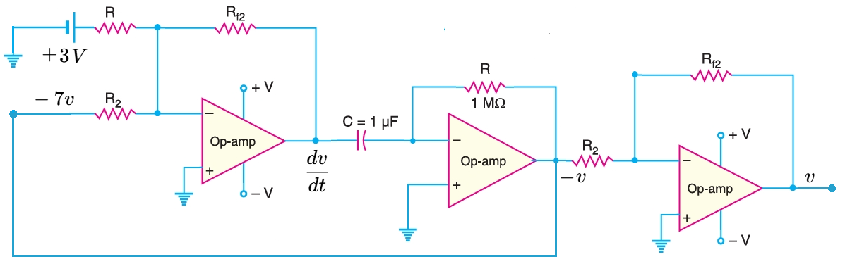
Always scale the output voltages to maintain linear operation and obtain an accurate solution which also prevent OP-AMP saturation. Choose the appropriate value for the saturation voltage \((V_{\text{SAT}})\) of the OP-AMP, and design an OP-AMP circuit to simulate the system by scaling the output voltage of integrator to unity, then passing it through a summing amplifier with a linear gain of \(-7\) and \(3 \,\text{Volts}\) d.c. source. This is one of many possible OP-AMP circuits that can be used to simulate the given differential equation
Three op amps are used, one as a summing amplifier, one as an integrator, and one as an inverting amplifier. The analog computer simulation was obtained by first taking the output of the integrator was chosen by choosing \(R = 1 \,\text{M}\Omega\) and \(C = 1 \mu\text{F}\), so that \(RC = 1 \,\text{second}\), which is fed back into the summing amplifier having two inputs. The first input is for the \(2 \,\text{V}\) dc input, and the second input is the feedback from the unity-gain inverting amplifier. The output of the summing amplifier will be fed into the integrator circuit.
Solve:
\[10\,\frac{d^{2}v(t)}{dt^{2}} + 400\,\frac{dv(t)}{dt} - 100\, v(t) = 500\, V\]
The first step is to algebraically solve for the highest-order derivative, \(d^{2}v/dt^{2}\):
\[\frac{d^{2}v}{dt^{2}} = -40\,\frac{dv}{dt} + 10\, v+50 \,V\]
The highest-order derivative is a combination or sum of lower derivatives and the smaller input voltage: \(dv/dt\), \(v\), and \(50\). Therefore, an inverting summing amplifier is needed to add the three terms, and these terms are forcing functions (or inputs) to the inverting summing amplifier.
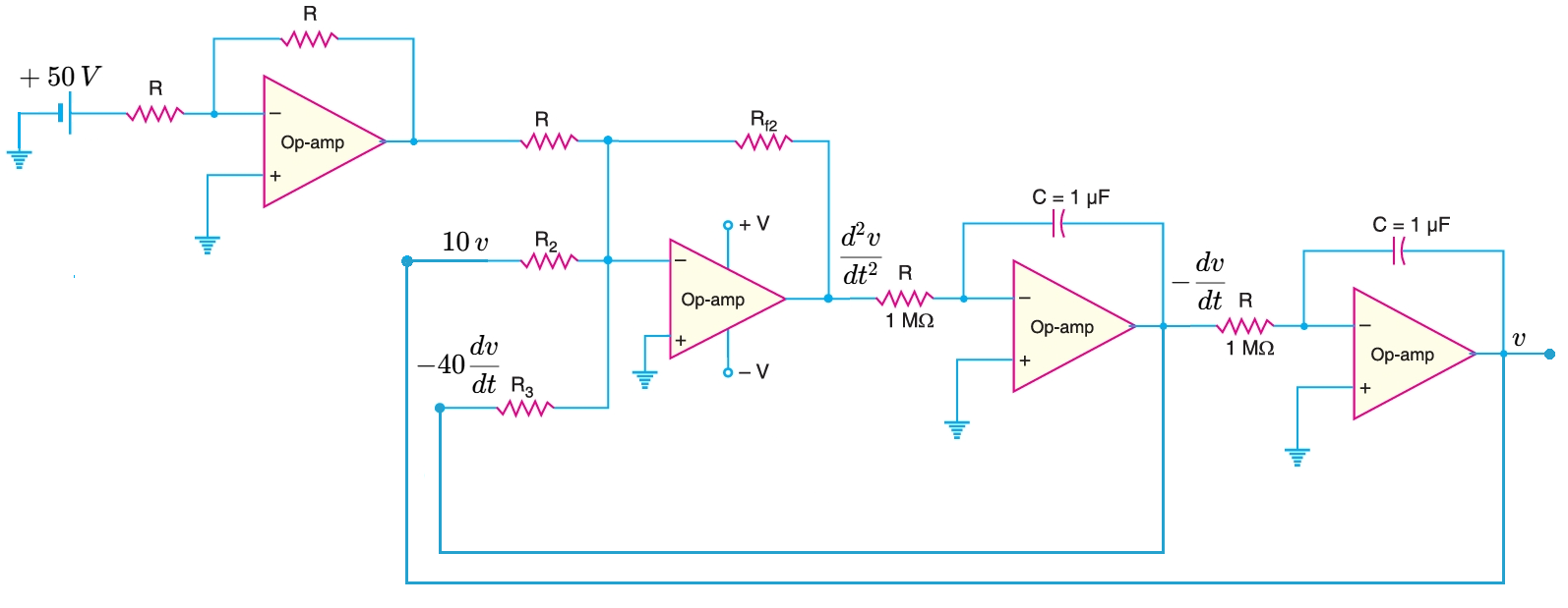
Use integrators to implement the block diagram, because the integral of a higher-order derivative is the derivative one order lower. For this example, integrate the second derivative, \(d^{2}v/dt^{2}\), to give you the first derivative, \(dv/dt\). As shown here, the output of the inverting summing amplifier is the second derivative (which is also the input to the first integrator). The output of the first inverting integrator is the negative of the first derivative \(dv/dt\) and serves as the input to the second inverting integrator. With the second inverting integrator shown in the figure, integrate the negative of the first derivative, \(–dv/dt\), to give you the desired output, \(v(t)\).
Take the integrator outputs, scale them, and feed them back into a summing amplifier (summing amplifier). The second derivative consists of a sum of three terms, so this is where the op amp inverting summing amplifier comes in. One of the inputs is a constant \(50\) volts to the summing amplifier, which will serve as an input voltage (or driving) source. The \(50\) volts at the input are fed to one of the summing amplifier inputs, with a gain of \(1\). The output of the first integrator is the first derivative of \(v(t)\), with a weight of \(40\), and is fed to the second input of the inverting summing amplifier. The output of the second integrator is fed to the third input to the inverting summing amplifier with a weight of \(10\). This completes the block diagram.
Solve:
\[\frac{d^{2}v}{dt^{2}}- 4\,\frac{dv}{dt} + 5\,v = 0\]
The analytical solution for this example is given below:
\[\frac{d^{2}v}{dt^{2}}= 4\,\frac{dv}{dt} -5\,v \]
Hence, multiply the first derivative \(dv/dt\) by \(4\) and multiply \(v\) by \(5\). Sum them as shown in the block diagram.
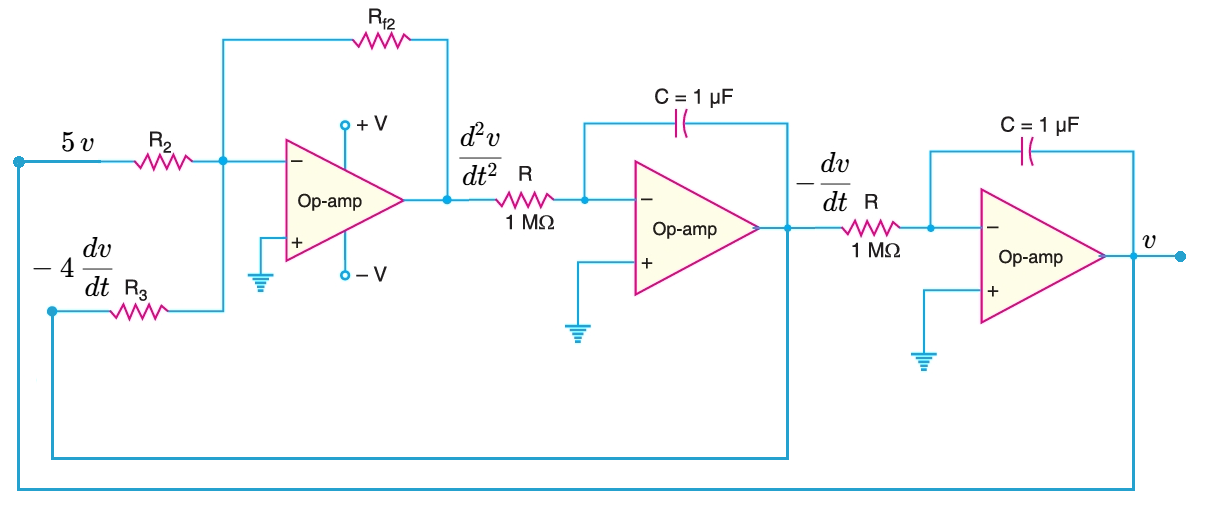
To simplify the design, set each integrator's gain to \(–1\). You need two more inverting amplifiers to get the signs right. Use the summing amplifier to achieve the gains of \(4\) and \(5\). Design the circuit to implement the block diagram.