Kirchhoff's laws
Circuit analysis is designed to find the voltage across or the current through any circuit element, and if need be the power consumed by its resistances or supplied by its sources. By far the most important aids to this analysis are Kirchhoff's two laws. They are fundamental to circuit analysis, and with them, and the current and voltage relations for circuit elements
The two laws are:
- Kirchhoff's voltage law
- Kirchhoff's current law
Kirchhoff's voltage law
The algebraic sum of the voltages at any instant around any loop in a circuit is zero.
Symbolically,
\[\sum~v= 0 \]
Kirchhoff's voltage law is a consequence of the principle of energy conservation; so frequent is its use in circuit theory that it is usually abbreviated to KVL.
Kirchhoff's current law
The algebraic sum of the currents at any instant at any node in a circuit is zero.
Symbolically,
\[\sum~i= 0 \]
KCL - its usual abbreviation - is a result of the principle of charge conservation
Illustrating Kirchhoff s laws.
The voltage law is used on loops ABCDEF A and ABEFA. The current law is used at node B.
A branch of a circuit is a path containing one circuit element. In figure AB is a branch, EF is not. A node is a point in a circuit where branches join. In figure, A and B are nodes, but F is not. There is also a node between the 4\(\Omega\) resistance and the \(4 V\) source.
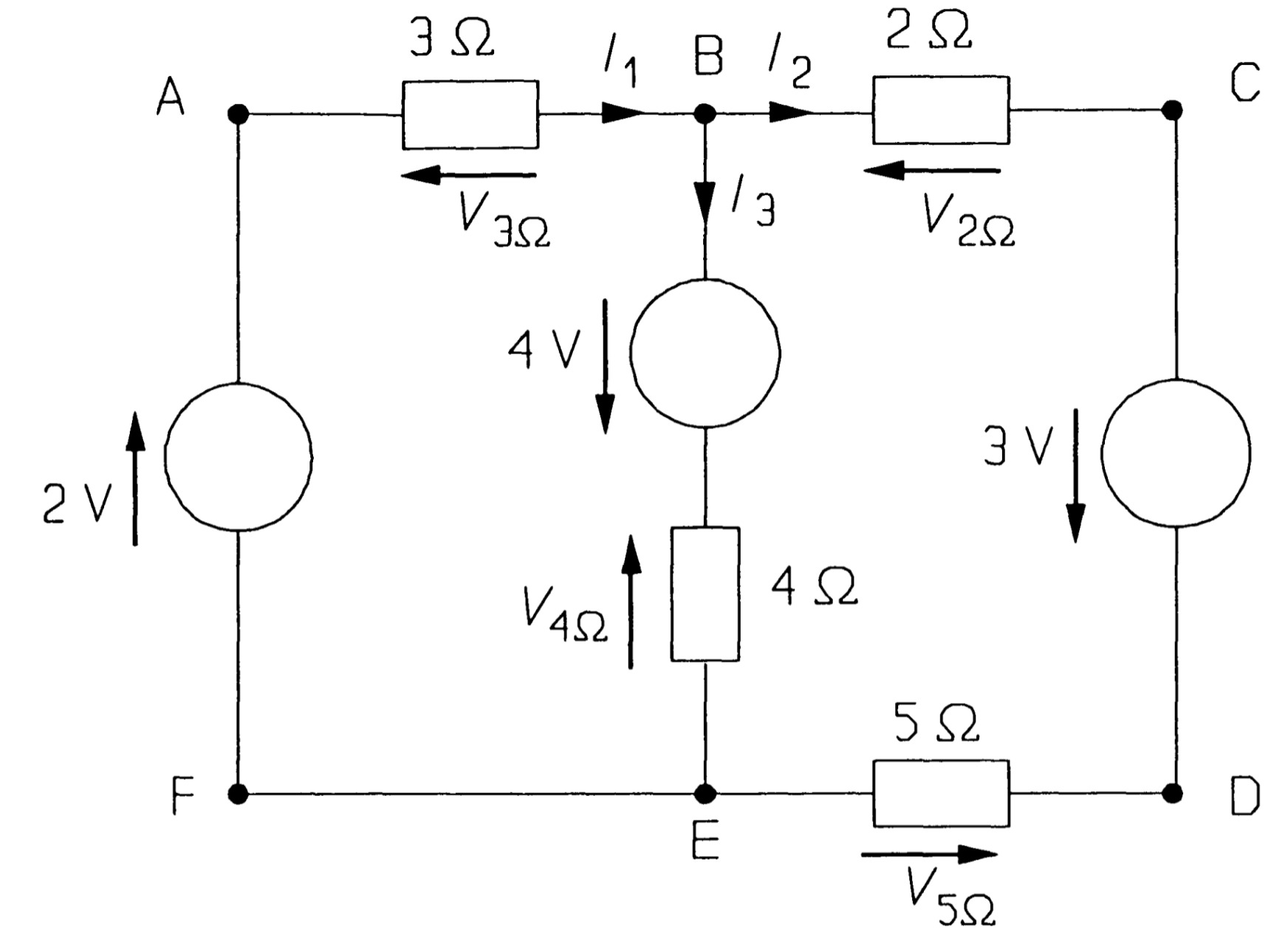
Selecting loop ABEFA, and taking clockwise-pointing voltages as positive and anticlockwise voltages as negative, we find:
\[ -V_{3\Omega}+4-V_{4\Omega}+2=0 ~~~~~~~~~~~~~~~~~~~~~~(1)\]
The choice of positive for clockwise voltages is arbitrary. Once you have assigned voltage arrows to the circuit elements (with voltage arrows on passive elements opposing the currents through them) you must wait until the analysis is complete to discover whether the polarity is 'right' (in which case the voltage will tum out to be positive) or 'wrong' (in which case the voltage will tum out to be negative). For loop ABCDEFA, KVL yields
\[-V_{3\Omega} -V_{2\Omega}+3-V_{5\Omega}+2=0 ~~~~~~~~~~~~~~~~~~~~(2)\]
and loop BCDEB produces
\[ -V_{2\Omega}+3-V_{5\Omega}+V_{4\Omega} -4=0 ~~~~~~~~~~~~~~~~~~~~~(3)\]
Note that subtracting equation 1 from equation 2 gives equation 3 - the application of KVL to this circuit produces only two independent equations. Voltages across the resistances can be found from Ohm's law; \(V_{3\Omega}\), for example, is \(3I_1\). Using this method equations 1 and 3 become
\[-3I_{1}-4I_{3}+6=0 ~~~~~~~~~~~~~~~~~~~~~~~~~~~(4)\\ -2I_{2}-5I_{2}+4I_{3}=0 ~~~~~~~~~~~~~~~~~~~~~~~~(5)\\ -7I_{2}+4I_{3}=0 ~~~~~~~~~~~~~~~~~~~~~~~~~~~(6)\]
Kirchhoff's current law is now needed to find a third equation for the unknown currents. If in figure we consider node B and take currents into the node as positive and currents out of the node as negative, then
\[I_{1}-I_{2}-I_{3}=0 ~~~~~~~~~~~~~~~~~~~~~~~~~~~~(7)\]
The three independent equations produced by application of Kirchhoff's and Ohm's laws to the circuit of figure are equation 4, 5 and 6, and solving these gives
\[I_1 = 1.017 A\]
\[I_2 = 0.279 A\]
\[I_3 = 0.738 A\]
The voltages across the resistances may be found from these currents with Ohm's law.
If inductances and capacitances are present Kirchhoff's laws can still be applied using the appropriate \(v-i\) relationships
\[v_L = L\frac{di}{dt}\]
and
\[v_C = \frac{1}{C} \int i~dt\],
which yield instantaneous values. (Kirchhoff's laws apply to direct, instantaneous and r.m.s. voltage and currents.) Kirchhoff's laws is used to decude useful results, starting with the addition of resistances, capacitances and inductances in series and in parallel.
Mesh analysis.
Mesh analysis applies KVL systematically to a circuit and produces simultaneous equations that may be solved to give the mesh currents. A mesh is a loop in a circuit with no loops inside it. Consider the circuit of the figure, which represents a domestic 2-phase supply common in North America. It contains three meshes: ABCDA, ADEFA, and CEDC; the large loop ABCDEF A is not a mesh as it can be divided into smaller loops. The meshes have been numbered 1, 2, and 3. Meshes one and two represent low-voltage circuits for lighting and appliances such as vacuum cleaners, hair dryers, etc., while mesh three represents a two-phase circuit for supplying relatively large loads. The 0.1\( \Omega \) resistances represent the wiring resistance.
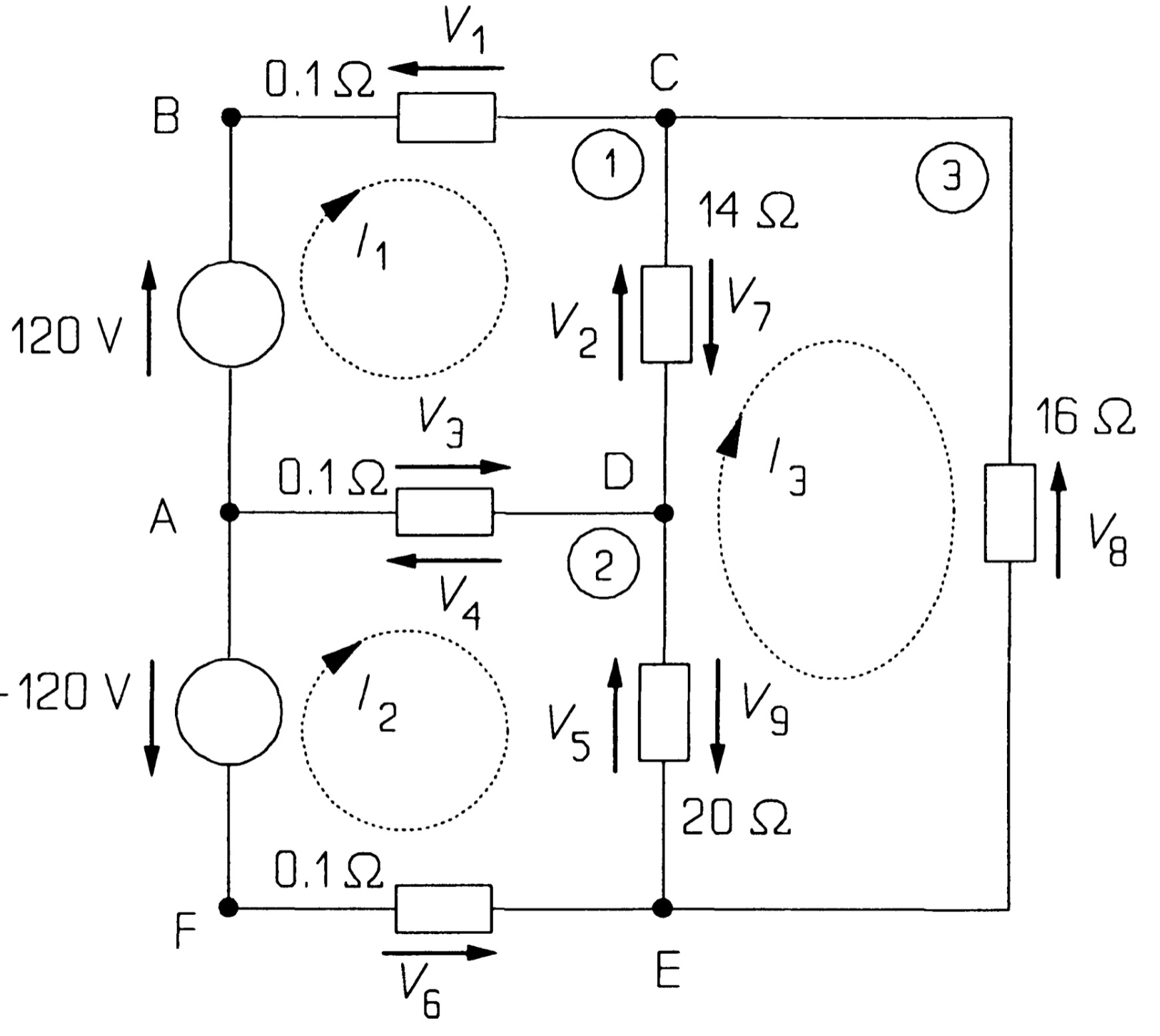
The first step in the analysis is to assign clockwise currents to each mesh: in this case, \( I_1 \), \( I_2 \), and \( I_3 \) to meshes 1, 2, and 3, respectively. The next step is to use KVL to find these currents. KVL around mesh 1 gives, with clockwise voltages taken as positive, anticlockwise negative:
\[ 120 - V_1 - V_2 - V_3 = 0 ~~~~~~~~~~~~~~~~~(1) \]
\( V_1 \) is the voltage across the 0.1\(\Omega\) resistance, which by Ohm's law is 0.1\( I_1 \). \( V_2 \) is the voltage across the 14\( \Omega \) resistance, which is not 14\( I_1 \), since the 14\( \Omega \) resistance is shared between meshes, and the resultant current flow from C to D must be \( (I_1 - I_3) \). \( V_2 \) must therefore be 14\( (I_1 - I_3) \). \( V_3 \) is the voltage across the middle 0.1\( \Omega \) resistance (the common wire for the two phases), which is shared between meshes 1 and 2. \( V_3 \) must then be 0.1\( (I_1 - I_2) \) and equation 1 becomes
\[ 120-0.1I_1 -14(I_1 - I_3)-0.1(I_1 - I_2)=0 ~~~~~~~~~~~~~~~~~(2) \]
or,
\[ 14.2I_1 - 0.1I_2 - 14I_3 = 120 ~~~~~~~~~~~~~~~~~(3) \]
after rearranging terms.
The use of KVL in mesh 2 yields
\[ -(-120) - V_4 - V_5 - V_6 = 0 ~~~~~~~~~~~~~~~~~(4) \]
The -120 V source points anticlockwise and is written -(-120) in equation 4 (if in doubt, reverse the arrow and the sign on this source, which leaves its value unchanged). \( V_4 \), the voltage across the middle 0.1 \( \Omega \) resistance, is 0.1 \( (I_2-I_1) \) by Ohm's law \( (V_4 = -V_3) \). \( V_5 \) is the voltage across the 20 \( \Omega \) resistance, and must be 20 \( (I_2-I_3) \) by Ohm's law, while \( V_6 \) is 0.1\( I_2 \), so that the equation becomes
\[ 120 - 0.1(I_2-I_1)-20(I_2-I_3)-0.1 I_3=0 ~~~~~~~~~~~~~~~~~(5) \]
which rearranges to
\[ -0.1I_1, + 20.2I_2 - 20I_3 = 120 ~~~~~~~~~~~~~~~~~(6) \]
Mesh 3 gives
\[V_7+V_8+V_9=0 ~~~~~~~~~~~~~~~~~(7)\]
Again, the voltages are found by using Ohm's law:
\[ V_7 = 14(I_3 - I_1) ~~~~~~~~~~~~~~~~~(8)\], \[ V_8 = 16I_3 ~~~~~~~~~~~~~~~~~(9)\] and \[ V_9 = 20(I_3 -I_2) ~~~~~~~~~~~~~~~~~(10)\].
Then, equation 7, after rearranging, is
\[ -14I_1 - 20I_2 + 50I_3 = 0 ~~~~~~~~~~~~~~~~~(11) \]
Three meshes have produced three equations, numbered 12, 13 and 14:
\[14.2I_1 - 0.1I_2- 14I_3 = 120 ~~~~~~~~~~~~~~~~~(12)\] \[ -0.1I_1 + 20.2I_2- 20I_3 = 120~~~~~~~~~~~~~~~~~(13)\] \[ -14I_1 - 20I_2 + 50I_3 = 0 ~~~~~~~~~~~~~~~~~(14)\]
Three meshes have produced three equations represented in matrix form:
\[ \begin{bmatrix} 14.2 & -0.1 & -14\\ -0.1 & 20.2 & -20\\ -14 & -20 & 50 \end{bmatrix} \begin{bmatrix} I_1 \\ I_2 \\ I_3 \end{bmatrix} = \begin{bmatrix} 120 \\ 120 \\ 0 \end{bmatrix} \]
And there are three unknown mesh currents. The solution is \( I_1 = 23.1 \) A, \( I_2 = 20.6 \) A and \( I_3 = 14.7 \) A.
The currents through the 14\( \Omega \) and 20\( \Omega \) loads are \( I_1 - I_3 (= 8.4 A) \) and \( I_2 -I_3 (= 5.9 A) \), while the common wire carries a relatively small current \( I_1 -I_2 (= 2.5 A) \). The power consumed by the 14\( \Omega \) load is \( 14 \times 8.42 = 990 W\) , by the 20\( \Omega \) load is \( 20 \times 5.92 = 700 \) W, and the 16 \( \Omega \) load consumes \( 16 \times 14.72 = 3.5 kW\) .
Take note of the form of equations 12, 13, and 14: The first comes from applying KVL to mesh 1, so the coefficient of \( I_1 \) is opposite in sign to those of the other two currents. The second equation arises from applying KVL to mesh 2, so the coefficient of \( I_2 \) is positive and the rest negative. The third equation comes from mesh 3, so the coefficient of \( I_3 \) is positive, the others negative. If the unknown currents and voltages are assigned in the systematic way described, the signs of the current coefficients should always follow this pattern - check if they do not! With a little practice, the student will find it superfluous to put voltages across resistances and will be able to write down the current equations directly. Aided by a computer solution of simultaneous equations, an experienced student can solve a 7-mesh problem in two to three minutes and get it right the first time.
Nodal analysis
While mesh analysis employs KVL systematically, nodal analysis uses KCL to give a set of simultaneous equations from which all the nodal voltages may be derived. Voltages are assigned to each principal node of a network, principal nodes being points where three or more branches of a circuit join. Strictly, a node is the point at which two or more branches join, and a principal node is one where three or more branches join.
Consider the circuit of the figure. The (principal) nodes are A, C, D, and E, with node A being chosen as the reference node. (The reference node need not be at ground potential, nor at any particular place in the circuit: the choice is arbitrary.) Voltages are then assigned to the other nodes representing the potential differences between them and the reference node: these are \( V_1 \), \( V_2 \), and \( V_3 \) in the figure. We then apply KCL at nodes C, D, and E. At node C, taking the current out of the node to be positive, we see that
\[ I_1 + I_2 + I_3 = 0 ~~~~~~~~~~~~~~~~~(1)\]
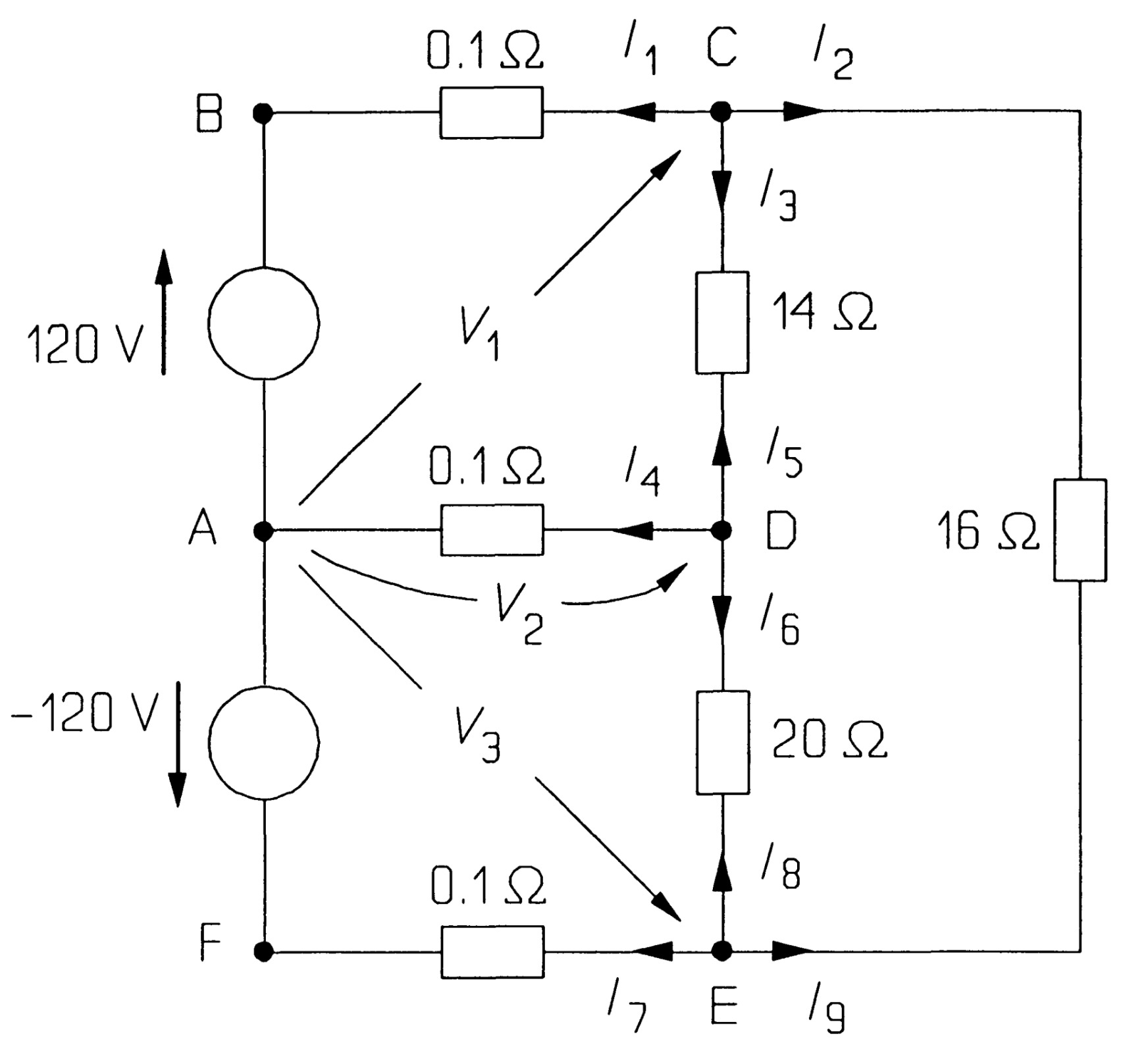
Now \( I_1 \) is the current through the uppermost 0.1\( \Omega \) resistance, which is given by Ohm's law as \( (V_1 - 120)/0.1 \) (make sure the sign is correct here!), since the voltage across the resistance is \( (V_1 - 120) \). Similarly, \( I_2 \) is \( (V_1 - V_3)/16 \) and \( I_3 \) is (V_1 - V_2)/l4. Equation 1 then becomes
\[ \frac{V_1 -120}{0.1}+\frac{V_1-V_3}{16}+\frac{V_1-V_2}{14}=0 ~~~~~~~~~~~~~~~~~(2) \]
At node D,
\[ I_4 + I_5 + I_6 = 0 ~~~~~~~~~~~~~~~~~(3)\]
Now \( I_4 = V_2 /0.1 \), as the middle 0.1\( \Omega \) resistance lies between the reference node A and node D, then \( I_5 = (V_2 - V_1)/14 \) (note that \( (I_5 = -I_3) \), but one should always give the currents at each node new identities, and work out afresh what they are) and \( ( I_6 = (V_2 - V_3)/20) \). Thus equation 3 is
\[ \frac{V_2}{0.1}+\frac{V_2-V_1}{14}+\frac{V_2-V_3}{20}=0 ~~~~~~~~~~~~~~~~~(4) \]
Finally, at node E
\[ I_7 + I_8 + I_9 = 0 ~~~~~~~~~~~~~~~~~(5)\]
where
\[ I_7 = (V_3 - (-120))/0.1 ~~~~~~~~~~~~~~~~~(6)\]
\[ I_8 = (V_3 - V_2)/20 ~~~~~~~~~~~~~~~~~(7)\]
\[ I_9 = (V_3 - V_1)/16 ~~~~~~~~~~~~~~~~~(8)\]
Substituting these values into equation 4 gives
\[ \frac{V_3 +120}{0.1}+\frac{V_3-V_2}{20}+\frac{V_3-V_1}{16}=0 ~~~~~~~~~~~~~~~~~(9) \]
Rearranging equations 2, 4 and 9 produces the three simultaneous equations.
\[ 10.13V_1 - 0.071V_2 - 0.0625V_3 = 1200 ~~~~~~~~~~~~~~~~~(10)\]
\[ -0.071 V_1 + 10.12V_2 - 0.05V_3 = 0 ~~~~~~~~~~~~~~~~~(11)\]
\[ -0.0625V_1 - 0.05V_2 + 10.11 V_3 = -1200 ~~~~~~~~~~~~~~~~~(12)\]
Three node equations are represented in matrix form:
\[ \begin{bmatrix} 10.13 & -0.071 & -0.0625\\ -0.071 & 10.12 & -0.05\\ -0.0625 & -0.05 & 10.11 \end{bmatrix} \begin{bmatrix} V_1 \\ V_2 \\ V_3 \end{bmatrix} = \begin{bmatrix} 1200 \\ 0 \\ 1200 \end{bmatrix} \]
The solution to the equations is \( V_1 = 117.7 \) V, \( V_2 = 0.24 \) V and \( V_3 = -118 \) V.
The form of these equations is worth remarking: the first comes from using KCL at node C, where the voltage relative to node A is \( V_1 \), and the only positive coefficient is that of \( V_1 \). The same pattern is followed in the other two equations. Any mistakes in sign should soon be noticed and put right if the equations are written in this systematic way. The solution to the equations is \( V_1 = 117.7 \) V, \( V_2 = 0.24 \) V and \( V_3 = -118 \) V. The voltage across the 14 \( \Omega \) load is \( 117.7- 0.24 = 117.5 \) V, and the current through it is \( 117.7/14 = 8.4 \) A, as before. The voltage across the 20 \( \Omega \) resistance is \( 0.24- (-118) = 118.2\) V, so the current through it is \( 5.9 \) A, and finally, the voltage across the 16 \( \Omega \) resistance is \( 117.7 -(-118) = 235.7 \) V, and the current through it is \( 14.7 \) A. The solution is, as it must be, the same as that found by mesh analysis earlier.
Maximum Power Transfer Theorem
When load is connected across a voltage source, power is transferred from the source to the load. The amount of power transferred will depend upon the load resistance. If load resistance \(R_{L}\) is made equal to the internal resistance \(R_{i}\) of the source, then maximum power is transferred to the load \(R_{L}\). This is known as maximum power transfer theorem and can be stated as follows :
Maximum power is transferred from a source to a load when the load resistance is made equal to the internal resistance of the source.
This applies to d.c. as well as a.c. power. To prove this theorem mathematically, consider a voltage source of generated voltage \(E\) and internal resistance \(R_{i}\) and delivering power to a load resistance \(R_{L}\). The current \(I\) flowing through the circuit is given by :
\[I = \frac{E}{R_{L}+R_{i}}\]
\[\text{Power delivered to load, } P = I^{2}R_{L} = \left(\frac{E}{R_{L}+R_{i}}\right)^{2}R_{L}\]
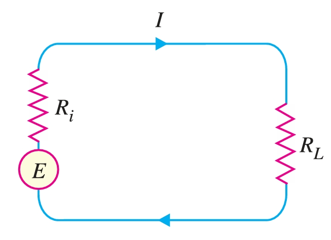
For a given source, generated voltage \(E\) and internal resistance \(R_{i}\) are constant. Therefore, power delivered to the load depends upon \(R_{L}\). In order to find the value of \(R_{L}\) for which the value of \(P\) is maximum, it is necessary to differentiate eq. (i) w.r.t. \(R_{L}\) and set the result equal to zero.
\[\frac{dP}{dR_{L}} = E^{2}\left[\frac{(R_{L}+R_{i})^{2}-2R_{L}(R_{L}+R_{i})}{(R_{L}+R_{i})^{4}}\right] =0\]
\[(R_{L}+R_{i})^{2}-2R_{L}(R_{L}+R_{i}) =0\ (R_{L}+R_{i}-2R_{L})=0\ (R_{i}-R_{L})=0\ R_{i}=R_{L}\]
i.e Load resistance = Internal resistance
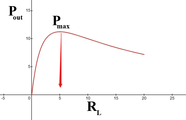
Thus, for maximum power transfer, load resistance \(R_{L}\) must be equal to the internal resistance \(R_{i}\) of the source. Under such conditions, the load is said to be matched to the source. Fig. 2 shows a graph of power delivered to \(R_{L}\) as a function of \(R_{L}\). It may be mentioned that efficiency of maximum power transfer is 50 % as one-half of the total generated power is dissipated in the internal resistance \(R_{i}\) of the source.
| Efficiency | = | \(\frac{\text{output power}}{\text{input power}} = \frac{I^{2}R_{L}}{I^{2}(R_{L}+R_{i})}\) |
| = | \(\frac{R_{L}}{2R_{L}} = \frac{1}{2} = 50 %\) |
Electric power systems never operate for maximum power transfer because of low efficiency and high voltage drops between generated voltage and load. However, in the electronic circuits, maximum power transfer is usually desirable. For instance, in a public address system, it is desirable to have load (i.e. speaker) matched to the amplifier so that there is maximum transference of power from the amplifier to the speaker. In such situations, efficiency is sacrificed at the cost of high power transfer.
Let us consider a generator develops 200 V and has an internal resistance of 100 Ω. The estimate of power transfer at various load are given in the table 1.
| \(R_{L} ~ (\Omega)\) | Load Current, \(I = \frac{E}{R_{L}+R_{i}}\) | Power delivered to \(R_{L}\), \(I^{2}R_{L}\) | Total Power, \(I^{2}(R_{L}+R_{i})\) | Efficiency (%) |
|---|---|---|---|---|
| \(100\) | \(\frac{200}{100+100}= 1.00 A\) | \((1.00)^{2} \times 100 = 100 ~watts\) | \(200 ~watts\) | \(50\) |
| \(200\) | \(\frac{200}{200+100}= 0.66 A\) | \((0.66)^{2} \times 200 = 88.8 ~watts\) | \(133.33 ~watts\) | \(66.60\) |
| \(200\) | \(\frac{200}{300+100}= 0.50 A\) | \((0.50)^{2} \times 300 = 75 ~watts\) | \(100 ~watts\) | \(75\) |
It is clear from the table 1 that although in case of \(R_{L} = R_{i}\), a large power (\(100 ~W\)) is transferred to the load, but there is a big wastage of power in the generator. On the other hand, when \(R_{L}\) is not equal to \(R_{i}\), the power transfer is less (\(75 ~W\)) but smaller part is wasted in the generator i.e., efficiency is high. Thus, it depends upon a particular situation as to what the load should be. If we want to transfer maximum power (e.g. in amplifiers) irrespective of efficiency, we should make \(R_{L} = R_{i}\). However, if efficiency is more important (e.g. in power systems), then internal resistance of the source should be consider ably smaller than the load resistance.
Thevenin's theorem
Thevenin's theorem states
Any two-terminal, linear network of sources and resistances may be replaced by a single voltage source in series with a resistance. The voltage source has a value equal to the open-circuit voltage appearing at the terminals of the network. The resistance value is the resistance that would be measured at the network's terminals when all the sources have been replaced by their internal resistances.
Any two-terminal network containing a number of e.m.f. sources and resistances can be replaced by an equivalent series circuit having a voltage source \(E_0\) in series with a resistance \(R_0\) where,
\(E_0\) = open circuited voltage between the two terminals. \(E_0\) = the resistance between two terminals of the circuit obtained by looking “in” at the terminals with load removed and voltage sources replaced by their internal resistances, if any.
Proceedure
- (i) Open the two terminals (i.e. remove any load) between which you want to find Thevenin equivalent circuit.
- (ii) Find the open-circuit voltage between the two open terminals. It is called Thevenin voltage \(E_{0}\).
- (iii) Determine the resistance between the two open terminals with all ideal voltage sources shorted and all ideal current sources opened (a non-ideal source is replaced by its internal resistance). It is called Thevenin resistance, \(R_{0}\).
- (iv) Connect \(E_{0}\) and \(R_{0}\) in series to produce Thevenin equivalent circuit between the two terminals under consideration.
- (v) Place the load resistor removed in step (i) across the terminals of the Thevenin equivalent circuit. The load current can now be calculated using only Ohm’s law and it has the same value as the load current in the original circuit.
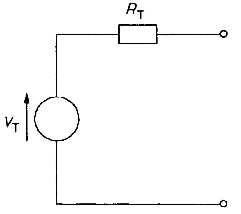
Thevenin's equivalent circuit is shown in figure. To replace complex networks by such a simple equivalent circuit can be highly convenient. For example let us find the Thevenin equivalent of the two-terminal network of figure. There are three steps in essence. First, is to determine the voltage across \(AB\). That is just the voltage across the \(4~\Omega\) resistance, which may be found by the voltage divider rule as the resistances are in series with the voltage source:
\[V_{AB} = V_{4\Omega} = 4 \times \frac{3}{6} = 2~V\]
This is the open-circuit voltage across \(AB\), and consequently the source voltage, \(V_T\), in the Thevenin equivalent circuit.
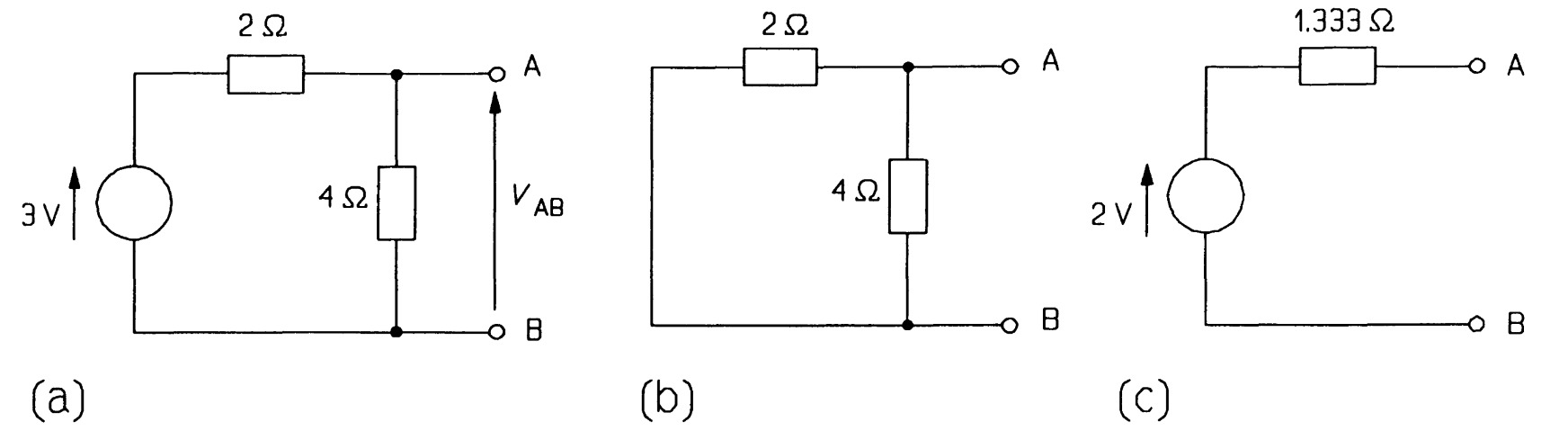
Secondly, the voltage source must be replaced by its internal resistance. As the voltage source is ideal and thus has zero internal resistance by definition, all this means is replace the voltage source by a short circuit. The circuit then becomes that of figure (b) simply two resistances in parallel when looked at from \(AB\). So, thirdly, we combine them by the product-over-sum rule:
\[R_{T} = \frac{2 \times 4}{2+4} = 1.333~\Omega \]
Hence the Thevenin equivalent of the network in figure (c). It is important to realise that the circuits of figures are equivalent only for measurements of current and voltage made at terminals \(A\) and \(B\), and nowhere else.
Find the current through the \(10~\Omega\) load resistance between \(A\) and \(B\) as given in the figure using Norton and Thevenin method.
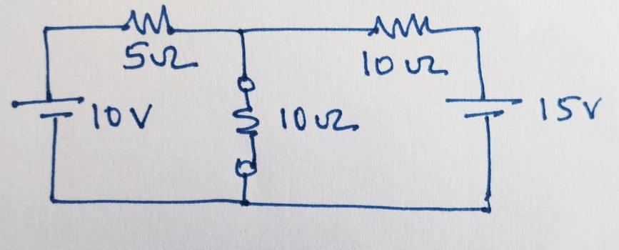
The first step using the Norton method is to remove the load resistance and short the terminal \(A\) and \(B\) and find the contibution of closed circuit current through terminals \(A\) and \(B\) for each of the voltage sources given. i.e., \(I_1\) for \(10~V\) and \(I_2\) for \(15~V\).
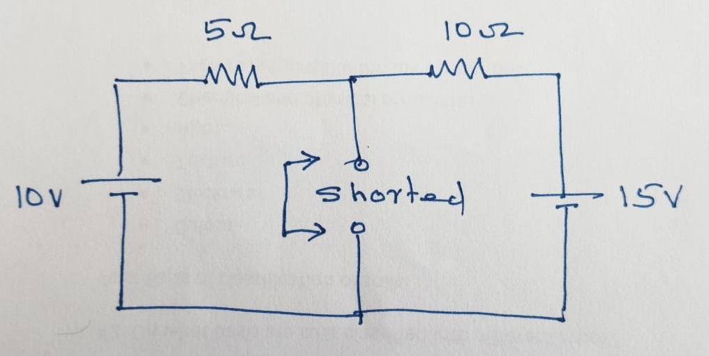
Hence, the \(I_1\) is calucalted as:
\[I_1 = \frac{10~V}{5~\Omega} = 2~A\]
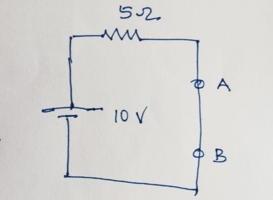
\(I_2\) is calculated as:
\[I_2 = \frac{15~V}{10~\Omega} = 1.5~A \]
Hence, the total closed circuit current through the terminal \(A\) and \(B\) is the Norton current, \(I_1\), which is:
\[I_N=I_1+I_2 = 2~ A + 1.5~A = 3.5~A\]
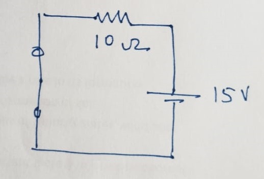
Now, let us estimate the Norton resistance, \(R_N\). The obtain the Norton resistance, the voltages should be shorted and current sources should be kept open. Here, we only have the voltage sources and the circuit given below shows the equivalent circuit with voltage lead shorted and the simplified form to estimate the \(R_N\).
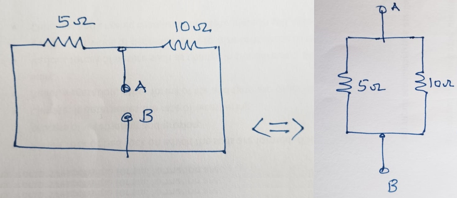
\(R_N\) is calculated as:
\[R_N = \frac{5\times 10}{5+10} = \frac{10}{3} = 3.333~\Omega \]
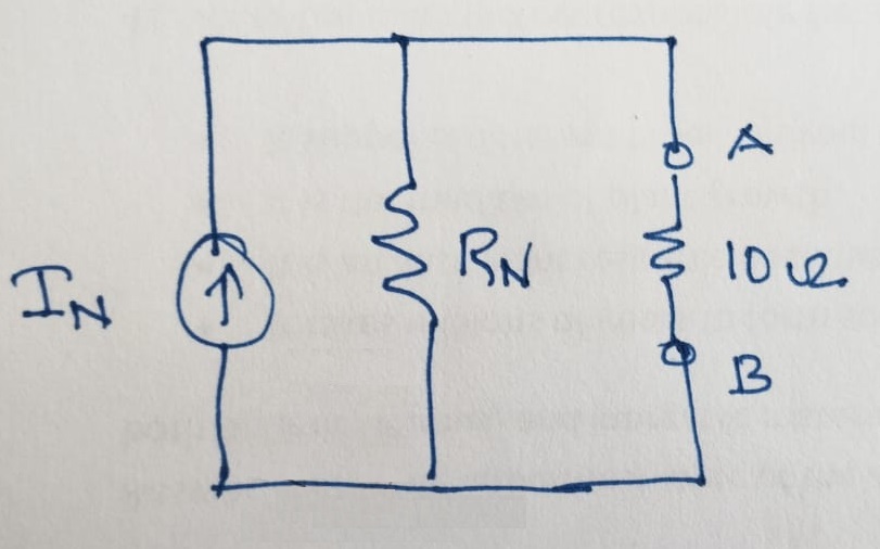
Now, we have the \(R_N\) and \(I_N\) as follows:
\[I_N = 3.5 ~A \\ R_N = 3.333 ~\Omega\]
The value of the current flowing through the load resistance (load current) is obtained by pluging back the \(6 ~\Omega\) resistance and by using the current division formula as follows:
\[I_L = I_N \left( \frac{R_N}{R_N+R_L}\right)\]
\[I_L = 3.5 ~A \left( \frac{3.333~\Omega}{[3.333+6]~\Omega}\right) = 1.25 ~A\]
Now, the total current flowing through the load resistance of \(6 ~\Omega\) is:
\[I_L = 1.25 ~A\]
The Thevenin voltage, \(V_{TH}\) is obtained from \(I_N\) and \(R_N\) as:
\[V_{TH}=I_N \times R_N \\ V_{TH}= 3.5 ~A \times 3.333 ~\Omega = 11.667 ~V \]
Now, let us Thevanize the same circuit as given below. Here, the terminals \(A\) and \(B\) should be kept open after removing the load resistance \(R_L\) to find the open circuit voltage due to each of the voltage sources given seperately.
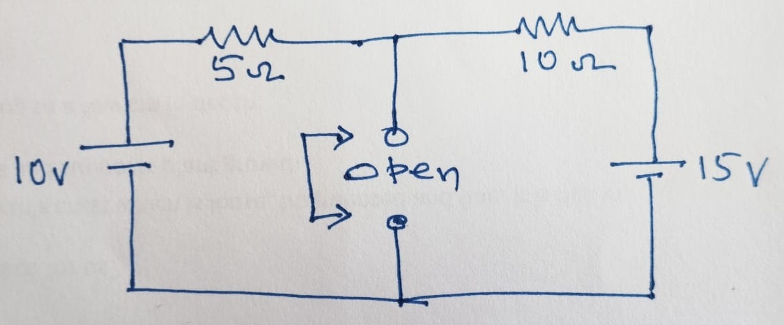
The contribution of open circuit voltage due to 10 V is calculated as:
\[V_1 = \frac{10 ~V}{10~\Omega + 5~\Omega}\times 10 ~\Omega = 6.667~V\]
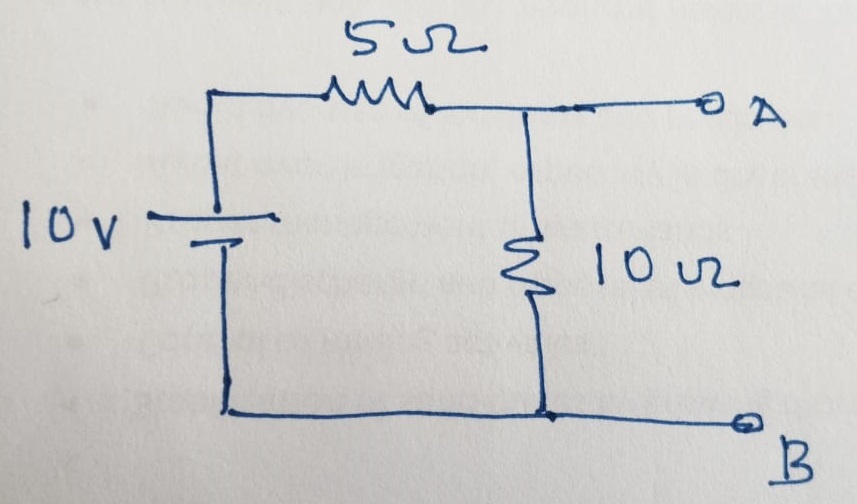
The contribution of open circuit voltage due to 15 V is calculated as:
\[V_1 = \frac{15 ~V}{10~\Omega + 5~\Omega}\times 5 ~\Omega = 5.00 ~V\]
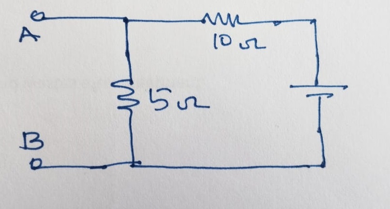
The total contribution of open circuit voltage due to 10 V and 15 V is calculated as:
\[V_{TH} = V_1 +V_2 = 6.667 + 5.00 ~V = 11.667 ~V\]
while,
\[R_N = R_{TH}\]
Hence,
\[R_{TH} = 3.333~\Omega \]
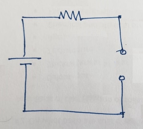
Now, the total current flowing through the load resistance of \(6 ~\Omega\) will be obtained as:
\[I_L = \frac{11.667 ~V}{3.333~\Omega + 6~\Omega} = 1.25 ~A\]
Norton's theorem
Norton's theorem is a useful complement to Thevenin's:
Any two-terminal, linear network of sources and resistances may be replaced by a single current source in parallel with a resistance. The value of the current source is the current flowing between the terminals of the network when they are short-circuited. The value of the resistance is the resistance measured at the terminals of the network when all sources have been replaced by their internal resistances.
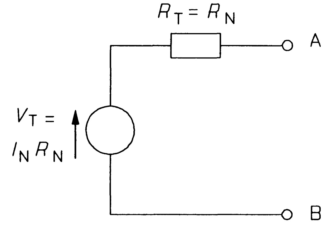
Norton's equivalent circuit is shown in figure.
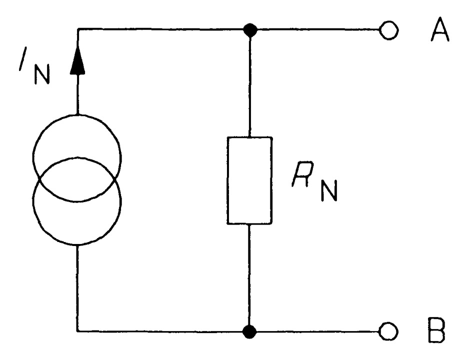
Any network having two terminals \(A\) and \(B\) can be replaced by a current source of output IN in parallel with a resistance \(R_N\).
- (i) The output \(I_N\) of the current source is equal to the current that would flow through AB when terminals \(A\) and \(B\) are short circuited.
- (ii) The resistance \(R_N\) is the resistance of the network measured between terminals \(A\) and \(B\) with load (\(R_L\)) removed and sources of e.m.f. replaced by their internal resistances, if any.
Norton’s theorem is converse of Thevenin’s theorem in that Norton equivalent circuit uses a current generator instead of voltage generator and resistance \(R_N\) (which is the same as \(R_0\)) in parallel with the generator instead of being in series with it.
Any two-terminal network of sources and resistances may be replaced by this AB. Since Thevenin's theorem applies to any two-terminal network, it must apply to Norton's equivalent circuit too. The Thevenin equivalent of Norton's circuit can be derived as follows: In figure the open-circuit voltage is that across \(R_{N}\), which must be \(I_{N}R_{N}\) since all the current from the source flows through it. Therefore
\[V_{T}=I_{N}R_{N}\]
The next step is to replace the source by its internal resistance - infinity for an ideal current source by definition - which amounts to open-circuiting an ideal current source. On doing this we are left with RN alone connected across AB, so the Thevenin resistance is identical to the Norton resistance:
\[R_{T}=R_{N}\]
Figure shows the transformation, which requires only the calculation of \(V_T=I_{N}R_{N}\), the open-circuit voltage of Norton's equivalent circuit. We must decide for ourselves whether we use the Norton or the Thevenin form of equivalent circuit. As a general rule one should use the Norton circuit to combine parallel sources and the Thevenin circuit to combine series sources.
Procedure
- (i) Open the two terminals (i.e. remove any load) between which we want to find Norton equivalent circuit.
- (ii) Put a short-circuit across the terminals under consideration. Find the short-circuit current flowing in the short circuit. It is called Norton current, \(I_{N}\).
- (iii) Determine the resistance between the two open terminals with all ideal voltage sources shorted and all ideal current sources opened (a non-ideal source is replaced by its internal resistance). It is called Norton’s resistance, \(R_N\). It is easy to see that \(R_N = R_0\).
- (iv) Connect \(I_{N}\) and \(R_{N}\) in parallel to produce Norton equivalent circuit between the two terminals under consideration.
- (v) Place the load resistor removed in step (i) across the terminals of the Norton equivalent circuit. The load current can now be calculated by using current-divider rule. This load current will be the same as the load current in the original circuit.
Hence, the current through the load resistance will be given by the Current division rule
\[I_L = I_N \left(\frac{R_N}{R_N + R_L}\right)\]
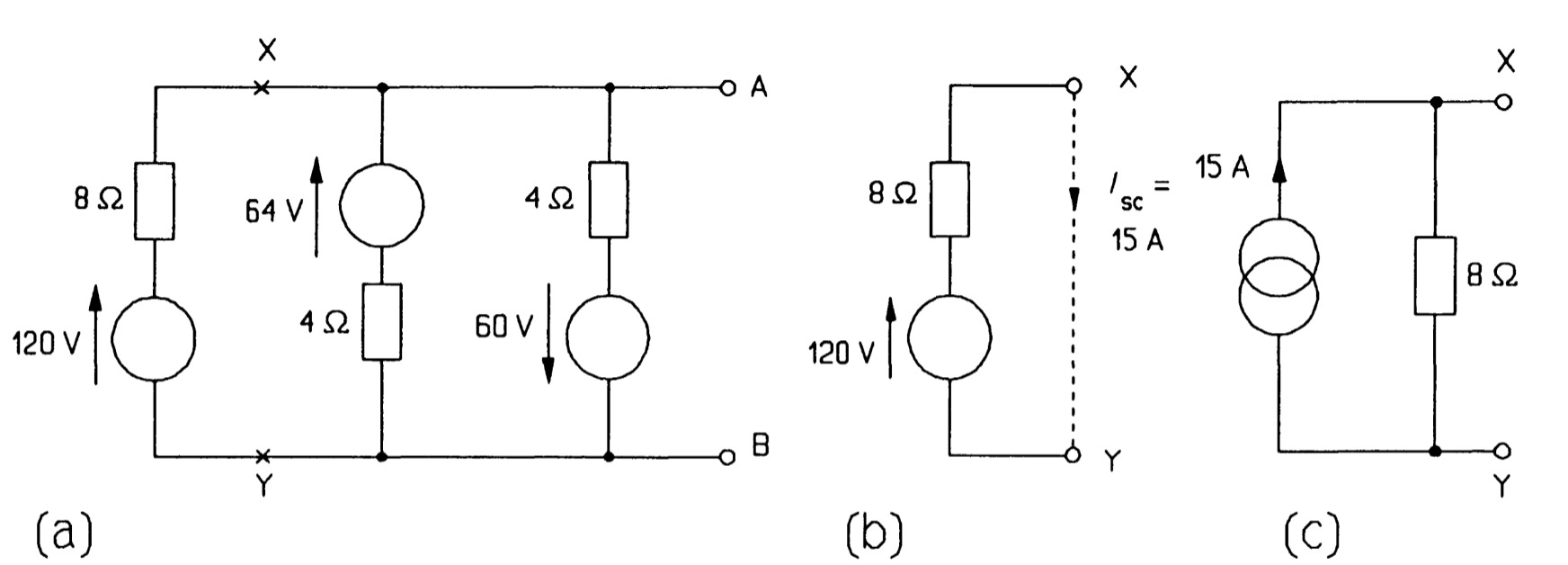
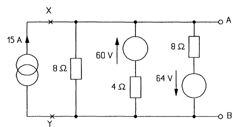
For example, consider the three generators in parallel in figure. We proceed by cutting the circuit at \(XY\) and looking at the source on the left by itself, as in figure. This source is in Thevenin form and must be transformed to the Norton form to enable us to add the parallel sources. The Norton source current is the current flowing through a short circuit across \(XY\), which is \(120/8 = 15 A\), by Ohm's law; and the Norton resistance is equal to the Thevenin resistance, \(8~\Omega\). So the Norton form of the 120 V source is as in figure. Note that the current arrow has the same direction as the voltage arrow of the original source. It is a good idea if in doubt to check this by examining which way current would flow through the short-circuited terminals. Having transformed the source we can re-attach it to the network at \(XY\) as in figure. The next voltage source is then transformed (it makes no difference which way round the voltage source and its series resistance are placed), and finally the one nearest to \(AB\). In the latter case the Norton equivalent must have its current arrow pointing down, like the voltage source it replaced. Figure shows the circuit at this stage.
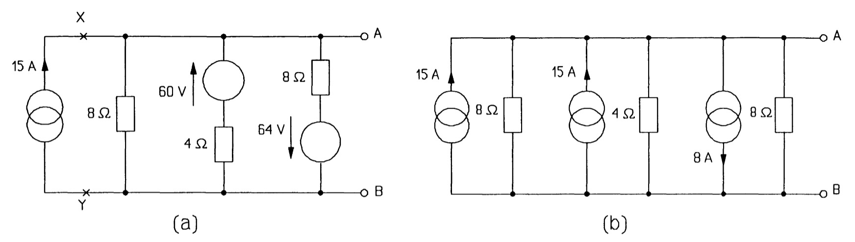
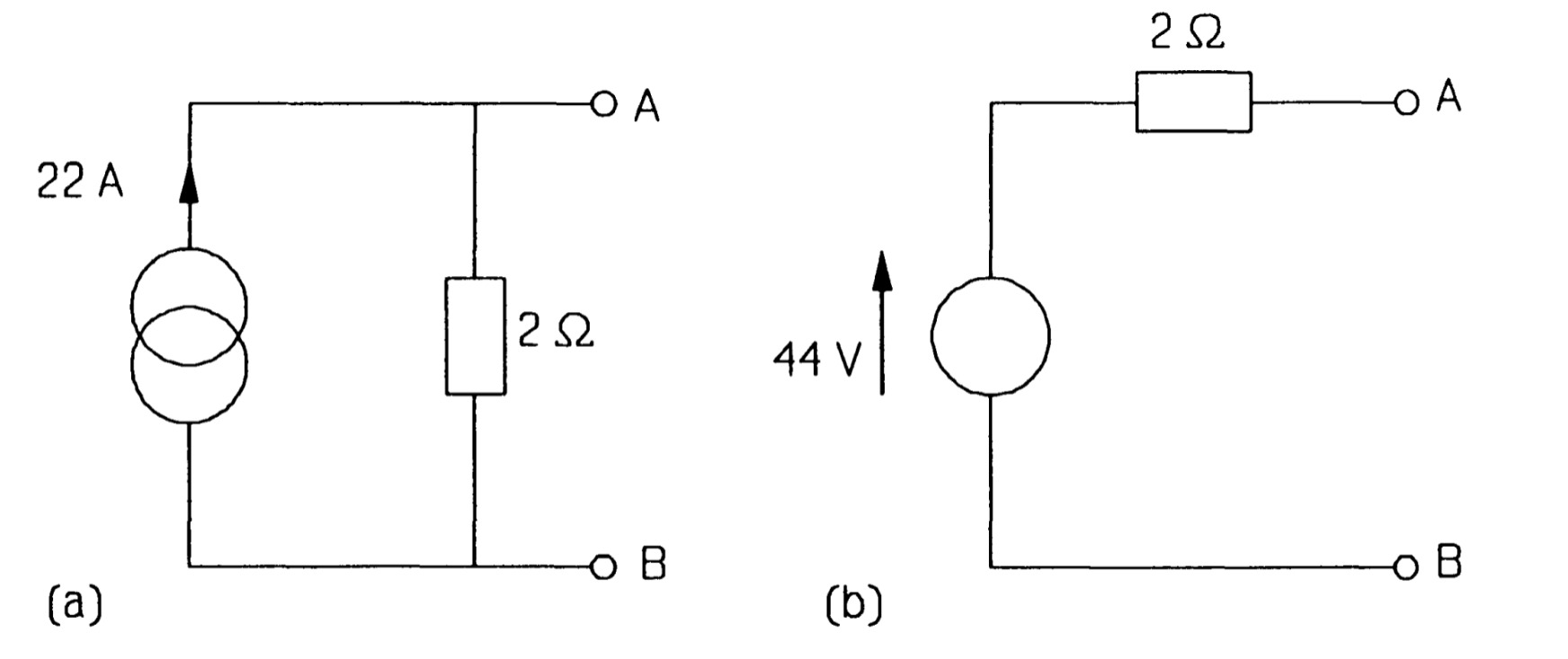
The three parallel current sources can now be added algebraically to give a single source of \(15 + 15- 8 = 22 A\). The third current source's value is subtracted from the other two as its direction is down and not up. Then the three parallel resistances in figure are combined to give a single 2\(\Omega\) resistance (by adding the reciprocals and taking the reciprocal of the result), giving the Norton circuit of figure . Finally the Norton circuit is turned into the Thevenin circuit of figure, using \(V_T = I_NR_N\).
Thevenin's and Norton's theorems enable us to take in principle any circuit inside a 'black box', make a measurement of the open-circuit voltage at its terminals, then the short-circuit current between them and from this represent the unknown contents of the box in the form of either equivalent circuit
Thevenin’s to Norton’s equivalent circuit
As mentioned previously, the Norton’s theorem is converse of Thevenin’s theorem and vice-versa, the Norton's equivalent circuit can be converted into Thevenin's equivalent circuit and back. The method of conversion is given below:
- (i) To convert Thevenin’s equivalent circuit into Norton’s equivalent circuit, \[I_N = E_0/R_0 ; \\ R_N = R_0\]
- (ii) To convert Norton’s equivalent circuit into Thevenin’s equivalent circuit \[E_0 = I_N R_N ; \\ R_0 = R_N\]
The superposition theorem
Sometimes it is helpful to consider separately the effects of sources on a particular part of the circuit; the superposition theorem lets us do that. It states
The current in any branch of a circuit, or the voltage at any node, may be found by the algebraic addition of the currents or voltages produced by each source separately. When the effect of one source is being considered, the other sources are replaced by their internal resistances.
Superposition is most useful when the sources are alternating sources of differing frequency, or a combination of direct and alternating sources, but we can illustrate the use of superposition with direct sources alone.
Consider the circuit of figure once more in which we wish to find \(V_{AB}\) using superposition. For this we must add the voltages produced across \(AB\) by each source in turn.
Taking the 120 V source first, we replace the other voltage sources by short circuits to obtain the circuit in figure. The parallel \(4~\Omega\) and \(8~\Omega\) resistances may be combined to give one of \(2.67~\Omega\), which is in series with the remaining 80 resistance, for a total resistance of \(10.67~\Omega\), so V, by the voltage divider rule must be \((2.67 /10.67) \times 120 = 30\) \(V\), as in figure
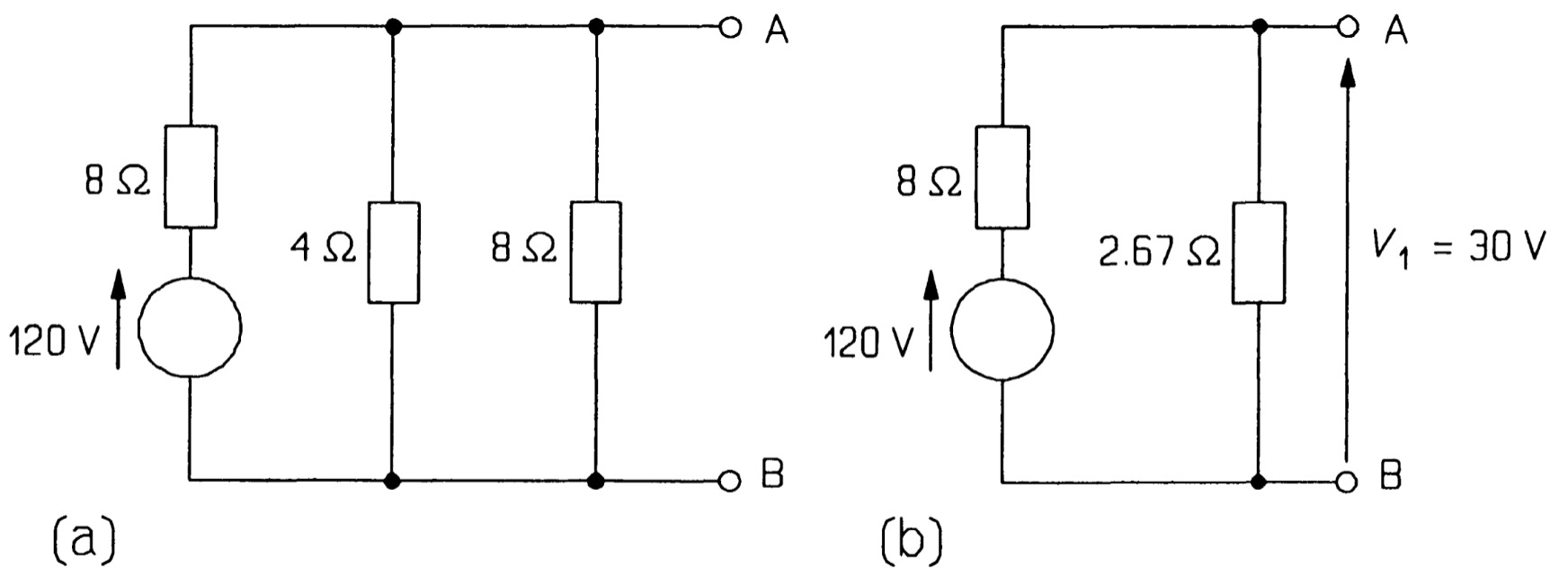
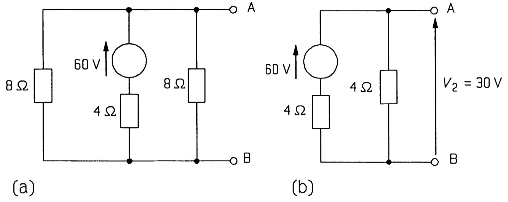
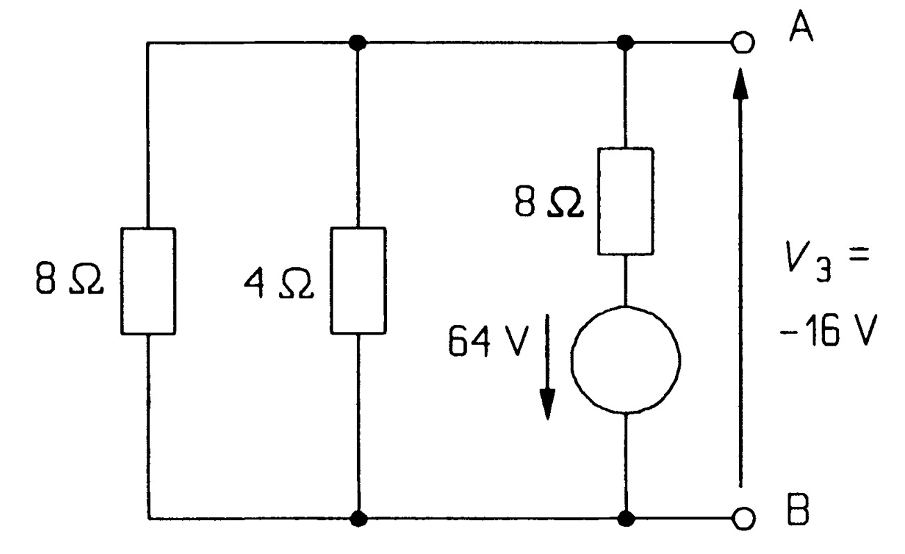
Proceeding in the same way to examine the effect of the 60V source we 'kill' the other two sources by replacing them with short circuits as in figure. The two \(8~\Omega\) resistances are in parallel as far as the \(60 V\) source is concerned, so they may be combined into a \(4~\Omega\) resistance. This is in series with the \(4~\Omega\) resistance next to the source, as in figure, so the voltage divider rule gives \(V_2\) as 30 V. The last step is to look at the effect of the 64 V source, as in figure. \(V_3\), the required voltage, is that across the parallel combination of \(8 ~\Omega\) and \(4~\Omega\) resistances, but as the 64 V source points to Band not A like the other two, \(V_3\) must be negative. Once again the parallel resistances combine to give one of \(2.67~\Omega\), so \(V_3\), calculated by the voltage divider rule, is
\[(2.67/10.67) \times (-64) V = -16 V\]
Summing:
\[V_{AB} = V_{1}+V_{2}+V_{3}\]