Introduction
Before any use can be made of electricity or of any electrical machine or device, it must form part of an electrical circuit. Even complex machines may be modelled by simple elements that, when assembled into a circuit in the right way, can be analysed and so predict the machine's behaviour. Accordingly, circuits are the foundation of any study of electrical or electronic engineering. We begin by defining simple circuit elements, then we shall incorporate them into circuits for analysis with the help of a number of laws and theorems. There are not many laws to remember- Ohm's law and Kirchhoff's laws are almost the only ones - but from these a number of theorems have been deduced to assist in circuit analysis. In this topic we shall primarily be concerned with direct currents and voltages (DC for short), but the principles developed will serve for analysing circuit behaviour with alternating currents and voltages (or AC). The circuit elements first considered are voltage and current sources and three passive elements: resistance, inductance and capacitance. Though simple these can be combined to form powerful equivalent circuits.
Sources
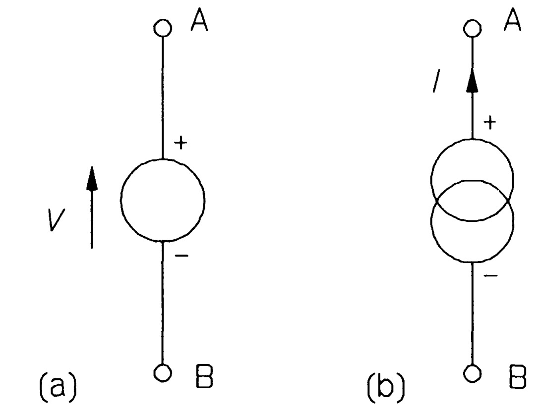
No electricity can flow in a circuit lacking a source, because sources are essential for supplying power. Practical sources include batteries, radio antennas and electro-mechanical generators, all of which can be modelled by ideal sources in combination with other circuit elements. Two sources are defined: the voltage source and the current source, the symbols for which are shown in figure
Sign convensions
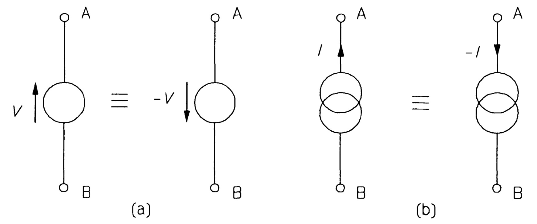
The voltage polarity signs are often omitted, since the arrow shows this more graphically. The value of the source voltage or current is written next to the arrow. An ideal voltage source will always maintain the voltage across its terminals, A and B, at the voltage indicated. An ideal current source will always pass the indicated current out of the positive terminal (A) and this current returns to the source at the negative terminal (B). A car battery makes quite a good approximation to an ideal voltage source for many purposes. Constant-current sources - within limits - can be made from a pair of transistors or from a single operational amplifier.
Passive circuit elements
For the moment we shall look at only three ideal passive circuit elements: resistance, capacitance and inductance.
Resistance
A resistor is a practical device that ideally possesses only resistance. An ideal resistor obeys Ohm's law:
\[V=IR\]That is, the voltage across a resistance is directly proportional to the current through it, resistance being the constant of proportionality. When I is in amperes \(A\) and V in volts \(V\), then R is in ohms (\(\Omega\)).
Ohm's law: current and voltage arrows are opposed when both current and voltage are positive
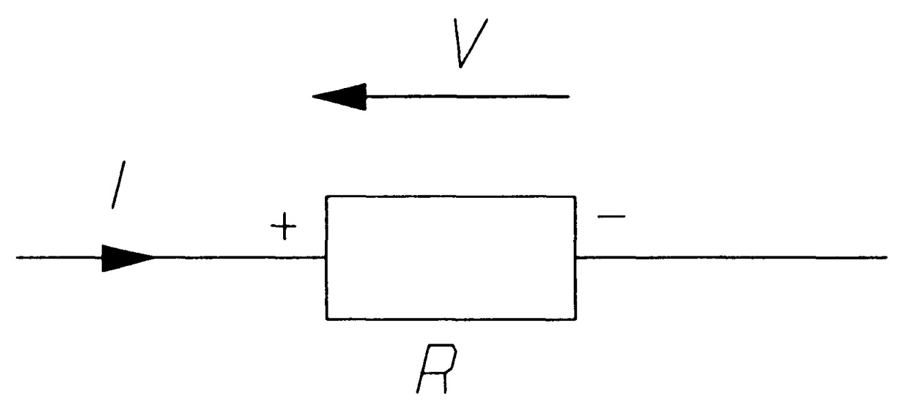
In figure, if the current through the resistance is in the direction shown, then the voltage arrow on the resistance must be opposed to it as indicated. If the arrow is reversed the voltage must be negative, following the sign convention previously described for sources. Ohm's law has been generalised and extended far beyond the scope originally intended for it, making it one of the most important laws
Capacitance
A capacitor is said to be a device for storing electric charge. Ideally it possesses only capacitance and no resistance or inductance. In figure, the current, /, flows into the positive plate and charges up the capacitance to a potential, V.
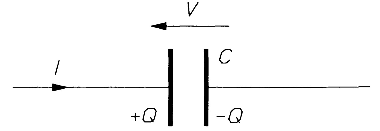
A capacitance with charge \(+Q\) on the positive plate and \(-Q\) on the negative. The total charge on the plates is zero. Charging results in the separation of positive and negative charges Current is the rate of flow of charge past a point in a circuit: \[i = \frac{dq}{dt} \] Here i and q are the instantaneous current and charge respectively. Substituting for q from equation yields \[i = C\frac{dv}{dt} \] which may be integrated to give the voltage across the capacitance: \[v=\frac{1}{C}\int i~dt\] Equation shows the voltage across a capacitance is the area under its current-time \(i-t\) graph divided by \(C\). The area under the \(i-t\) graph is the charge, \(Q\).
Inductance
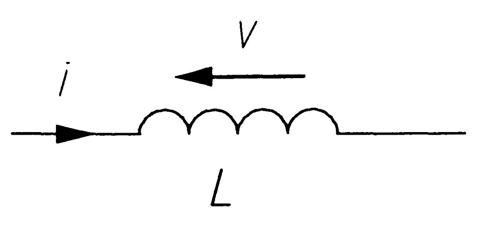
An ideal inductor possesses only inductance, which is sometimes called self inductance to distinguish it from mutual inductance. In figure an ideal inductor is shown. The voltage and current arrows are opposed, and the voltage is given by
\[v=L\frac{di}{dt}\]Equation indicates that there is no voltage across an inductance unless the current through it is changing. It also shows that if the current into the inductance is increasing, then the opposing voltage increases also. If the current is decreasing, the voltage is negative - in other words, the voltage arrow is reversed.
Mutual inductance
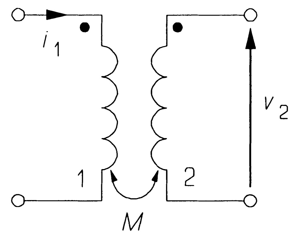
When two coils are wound onto a ferromagnetic core, or are in close proximity to each other, some of the magnetic flux produced by a one coil will link with the other coil, which is called coupling. In figure a changing current, \(i_1\), in coil 1 induces a voltage, \(v_2\), in coil 2. The current and voltage are related by \[v=M\frac{di_i}{dt}\] where M is the mutual inductance of the coils. A changing current, \(i_2\), in coil 2 would similarly produce a voltage, \(v_1\), in coil 1 of magnitude \(Mdi_2 /dt\). The dots indicate the winding direction, which is such that a positive current going into the dotted terminal will produce a positive voltage at the other dotted terminal. If the magnetic flux produced by one coil all links with the other coil, then it can be shown that \[M=\sqrt{L_1L_2}\] where \(L_1\), \(L_2\) are the self inductances of the coils. The coils are said to be perfectly coupled. If the coupling is not perfect then \[M=k\sqrt{L_1 L_2}\] \(k\), the coefficient of coupling, lies between \(0\) (no coupling) and \(1\) (perfect coupling).
Practical circuit elements
The circuit elements discussed so far have been ideal but practical circuit elements can be modelled from them. Some circuit elements are more nearly ideal than others; ideal sources, for example, cannot exist. Were we to short-circuit the terminals of an ideal voltage source, the current flowing would be infinite; and were we to open circuit the terminals of an ideal current source, the voltage across its terminals would be infinite. But at comparatively low frequencies capacitors and resistors are for practical purposes ideal.
The practical voltage source
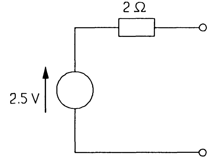
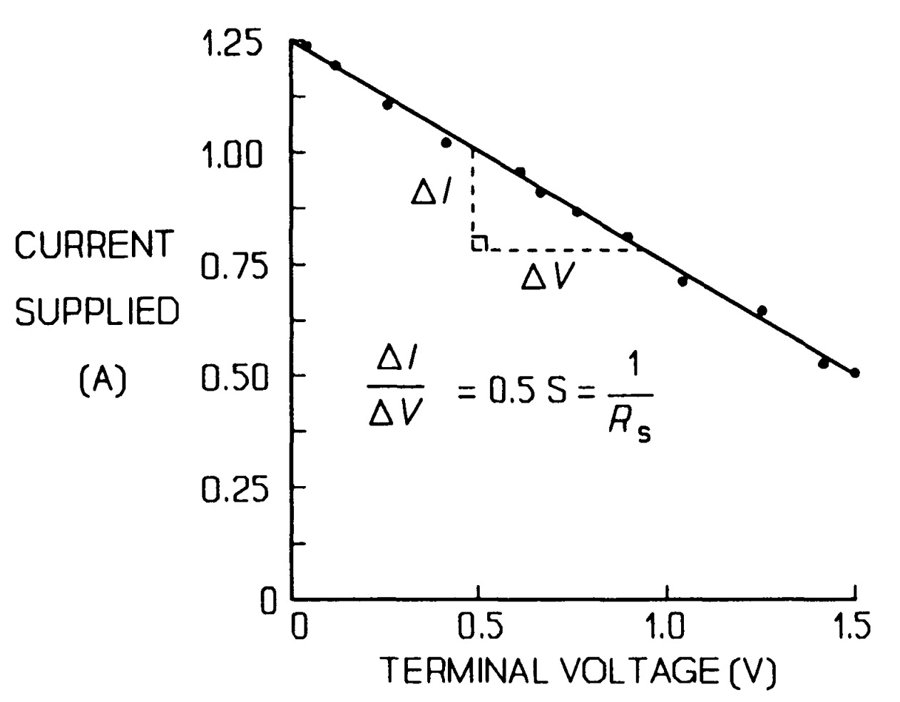
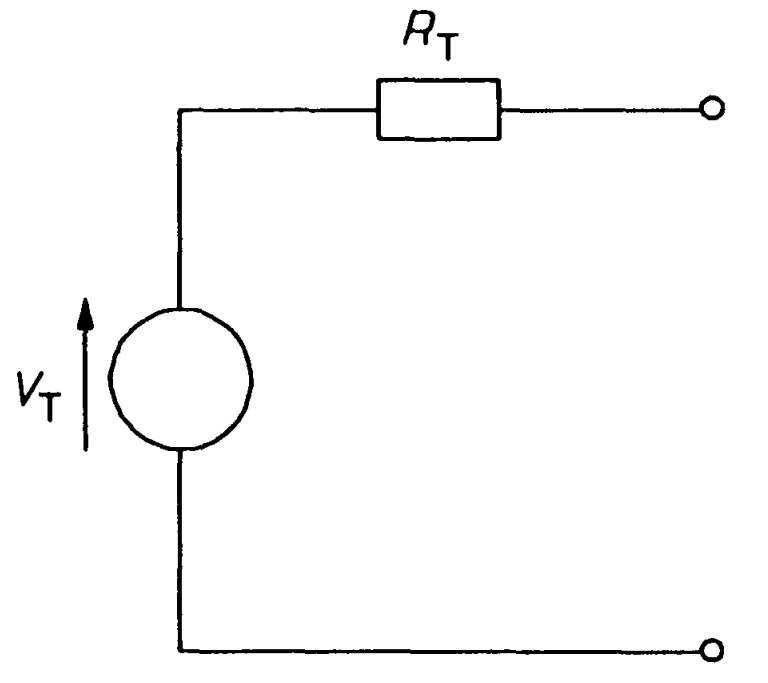
The model of a practical voltage source should be a resistance in series with an ideal voltage source as in figure.
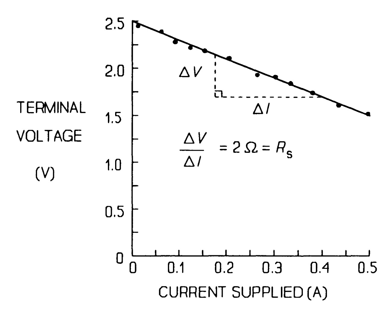
The ideal source's e.m.f. must be \(\2.5 V), the same as the open-circuit voltage of the battery while the resistance value must be given by the slope of the \(V-I\) graph (with the sign changed), or 2 \(\Omega\). This resistance is known as the internal resistance of the source. Then when the current drawn is \(0.5 A\), the internal resistance has a voltage across it of
\[V = IR = 0.5 \times 2 = 1 V\]The terminal voltage differs from the open-circuit voltage by this much when the battery is delivering \(0.5 A\).
A model of a practical voltage source. If the resistance were zero the source would be idea
The practical current source
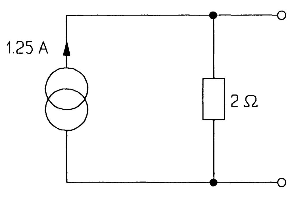
Some of the source current is being diverted through an internal resistance in parallel with the load across the terminal. Here it can be seen that the current supplied when the terminal voltage is zero - the short-circuit current - is 1.25 A, but when a load is connected across the terminals, the current falls and as it does so the voltage across the terminals rises.
A practical current source. When the resistance is infinite (or the conductance is zero), the current source is ideal
Practical resistors
Metal-film or carbon-film resistors commonly used in circuits and rated from \(\1/8 W) to \(2 W\) have very little capacitance or inductance- virtually negligible up to \(100 kHz\); wirewound resistors of higher wattage generally have a few \(pH\) of inductance and may be modelled as a small inductor in series with a resistance. Often of more serious concern is the temperature coefficient of resistance (sometimes known as the tempco) and the tolerance, that is how much the actual value of the resistance differs from the nominal value given by the colour-band code on the resistor. Practical resistors also have rated voltages and temperatures which must not be exceeded.
Practical capacitors
A practical capacitor has some leakage resistance which can be modelled as a resistance in parallel with a capacitance, as in figure. A model of a practical capacitor. In a high quality capacitor at relatively low frequencies, \(R_P\) may be \(1 G\Omega\) or more.
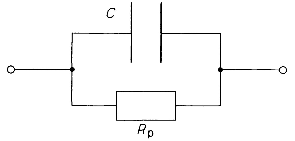
Leakage resistance is of two origins: surface leakage and internal (dielectric leakage); the latter is more important and both are dependent on frequency. The capacitors inductance may also need to be considered at frequencies above \(10~MHz\). The physical size of a capacitor depends on the type of construction, the capacitance and the working voltage. Electrolytic capacitors are polar (the terminal marked \(+\) must be connected to the more positive voltage) and have relatively high leakage (that is a lower parallel leakage resistance); however, they are cheap for high capacitance values.
Practical inductors
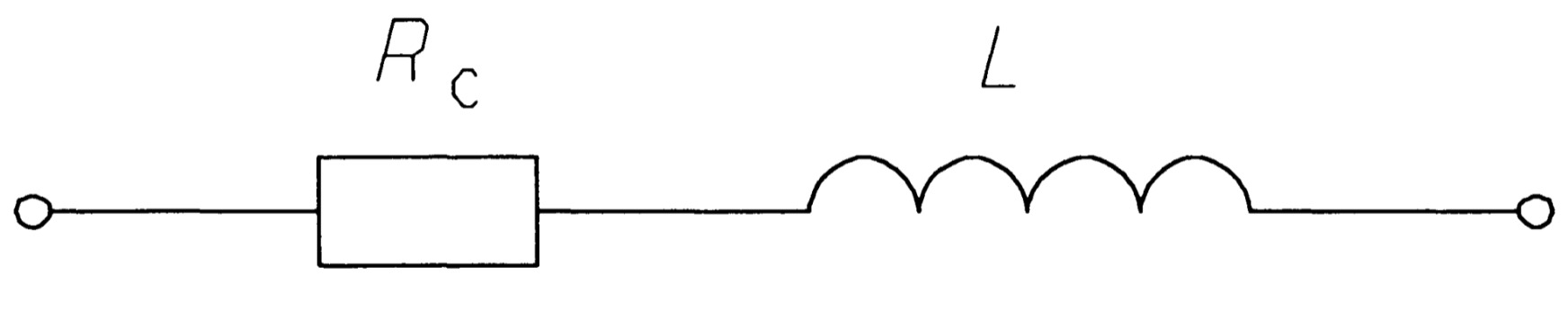
For many purposes it is possible to treat capacitors and resistors as ideal, but one can seldom do so with inductors: they must be modelled as an ideal inductor in series with a resistance as in figure. \(R_c\) is the resistance of the inductor to \(DC\).
Circuit analysis and Kirchhoff's laws
Circuit analysis is designed to find the voltage across or the current through any circuit element, and if need be the power consumed by its resistances or supplied by its sources. By far the most important aids to this analysis are Kirchhoff's two laws. They are fundamental to circuit analysis, and with them, and the current and voltage relations for circuit elements
The two laws are:
- Kirchhoff's voltage law
- Kirchhoff's current law
Kirchhoff's voltage law
The algebraic sum of the voltages at any instant around any loop in a circuit is zero.
Symbolically,
\[\sum~v= 0 \]Kirchhoff's voltage law is a consequence of the principle of energy conservation; so frequent is its use in circuit theory that it is usually abbreviated to KVL.
Kirchhoff's current law
The algebraic sum of the currents at any instant at any node in a circuit is zero.
Symbolically,
\[\sum~i= 0 \]KCL - its usual abbreviation - is a result of the principle of charge conservation
Illustrating Kirchhoff s laws.
The voltage law is used on loops ABCDEF A and ABEFA. The current law is used at node B.
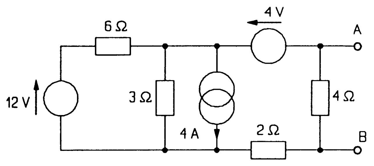
A branch of a circuit is a path containing one circuit element. In figure AB is a branch, EF is not. A node is a point in a circuit where branches join. In figure, A and B are nodes, but F is not. There is also a node between the 4\(\Omega\) resistance and the \(4 V\) source.
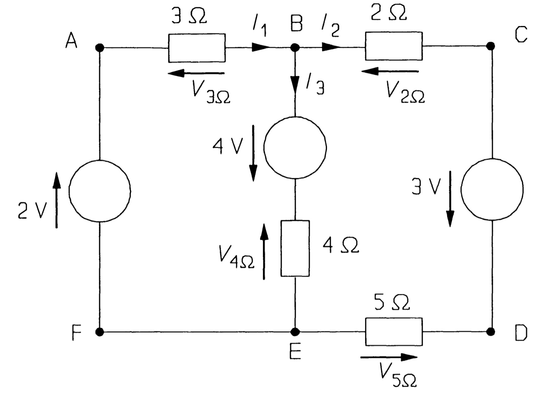
Selecting loop ABEFA, and taking clockwise-pointing voltages as positive and anticlockwise voltages as negative, we find:
\[ -V_{3\Omega}+4-V_{4\Omega}+2=0 ~~~~~~~~~~~~~~~~~~~~(1)\]The choice of positive for clockwise voltages is arbitrary. Once you have assigned voltage arrows to the circuit elements (with voltage arrows on passive elements opposing the currents through them) you must wait until the analysis is complete to discover whether the polarity is 'right' (in which case the voltage will tum out to be positive) or 'wrong' (in which case the voltage will tum out to be negative). For loop ABCDEFA, KVL yields
\[-V_{3\Omega} -V_{2\Omega}+3-V_{5\Omega}+2=0 ~~~~~~~~~~~~~~~~~~~~(2)\]and loop BCDEB produces
\[ -V_{2\Omega}+3-V_{5\Omega}+V_{4\Omega} -4=0 ~~~~~~~~~~~~~~~~~~~~(3)\]Note that subtracting equation 1 from equation 2 gives equation 3 - the application of KVL to this circuit produces only two independent equations. Voltages across the resistances can be found from Ohm's law; \(V_{3\Omega}\), for example, is \(3I_1\). Using this method equations 1 and 3 become
\[-3I_{1}-4I_{3}+6=0 ~~~~~~~~~~~~~~~~~~~~(4)\] \[-2I_{2}-5I_{2}+4I_{3}=0 ~~~~~~~~~~~~~~~~~~~~(5)\] \[-7I_{2}+4I_{3}=0 ~~~~~~~~~~~~~~~~~~~~(6)\]Kirchhoff's current law is now needed to find a third equation for the unknown currents. If in figure we consider node B and take currents into the node as positive and currents out of the node as negative, then
\[I_{1}-I_{2}-I_{3}=0 ~~~~~~~~~~~~~~~~~~~~(7)\]The three independent equations produced by application of Kirchhoff's and Ohm's laws to the circuit of figure are equation 4, 5 and 6, and solving these gives \(I_1 = 1.017 A\), \(I_2 = 0.279 A\), \(I_3 = 0.738 A\). The voltages across the resistances may be found from these currents with Ohm's law.
If inductances and capacitances are present Kirchhoff's laws can still be applied using the appropriate \(v-i\) relationships (\(v_L = L\frac{di}{dt}\) and \(v_C = C^{-1} \int i~dt\)), which yield instantaneous values. (Note that Kirchhoff's laws apply to direct, instantaneous and r.m.s. voltage and currents.) Many useful results are soon deduced from Kirchhoff's laws, starting with the addition of resistances, capacitances and inductances in series and in parallel.
Resistances in series
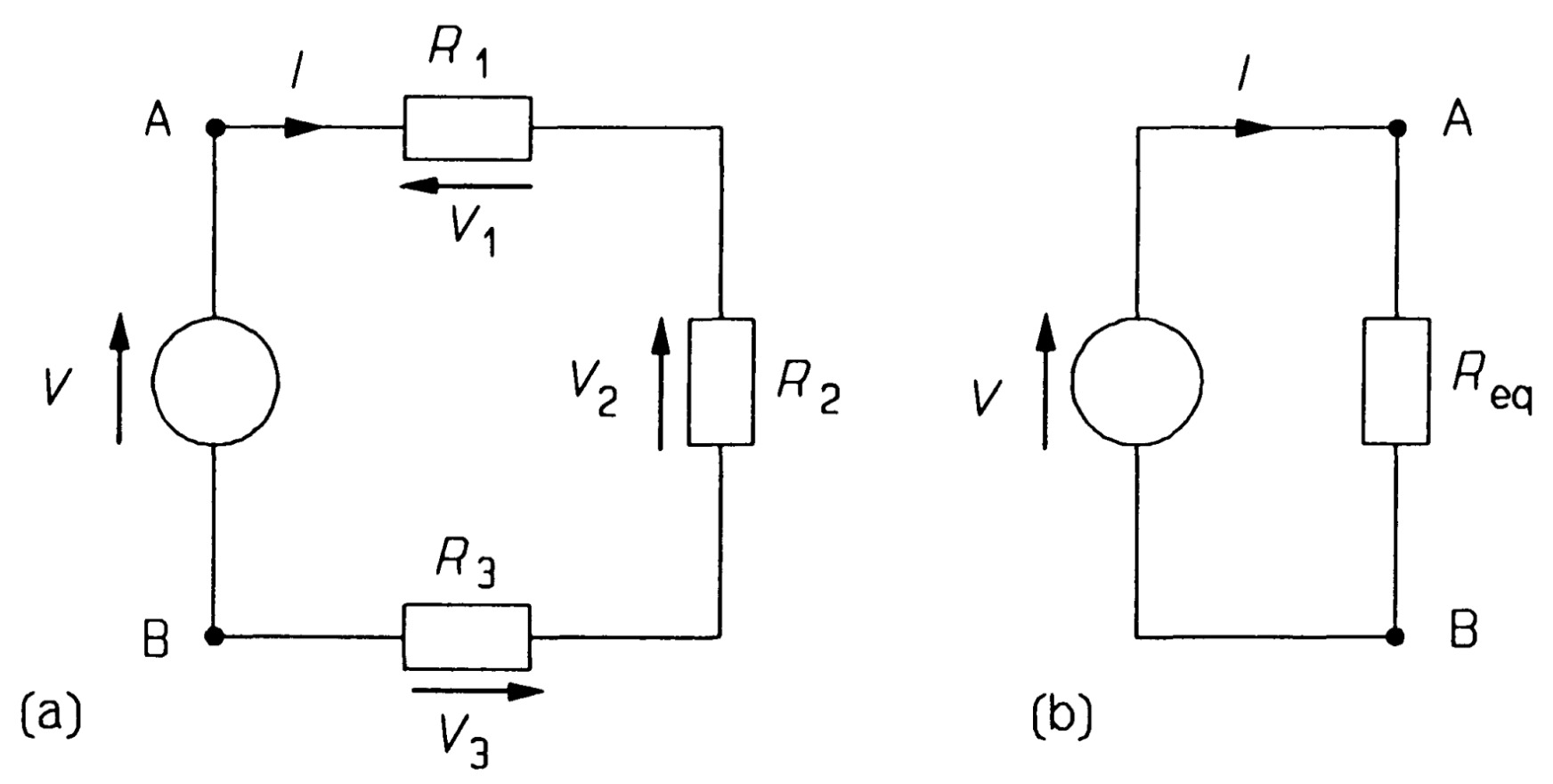
Looking at figure - three resistances in series - and applying KVL we find (1.22)
\[V- V_{1} - V_{2} - V_{3}=0\]But V1 = IR 1 and V2 = IR2 and V3 = IR3, and substitution into equation 1.22 yields
\[V=IR_{eq} = IR_{1} + IR_{2} + IR_{3} =I(R_{1} + R_{2} + R_{3})\]where
\[R_{eq} = R_{1} + R_{2} + R_{3}\]Since \(I = V/R_{eq}\), then
\[ V_{1}=\left(\frac{R_{1}}{R_{1} +R_{2} +R_{3}}\right) V = \left(\frac{R_{1}}{R_{eq}}\right) V \]which illustrates the voltage divider rule: the voltage across resistances in series divides in proportion to the value of each.
Conductances in parallel:
Conductance is the reciprocal of resistance:
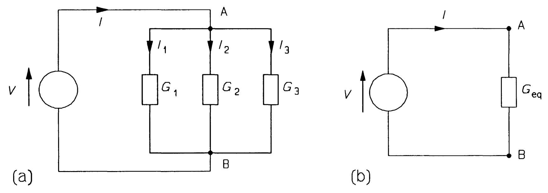
\[G = \frac{1}{R}\]The units of conductance are Seimens (S). Taking the circuit in the figure which has three conducatances in parellel, we can apply KCL at node A to obtain,
\[I=I_1 +I_2+I_3\]But the voltage across each conductance is the same and Ohm's law gives
\[V=I_1R_1=I_2R_2=I_3R_3\]Thus \(I_1=VG_1\), \(I_2 =VG_2\), \(I_3=VG_3\) etc., and substitution into equation leads to
\[I = VG_{eq} = VG_1+VG_2+VG_3 = V(G_1+G_2+G_3)\]Hence, we add parallel conductances as
\[G_{eq} = G_1 + G_2 + G_3\]If we let the equivalent resistance be \((R_{eq}= 1/G_{eq})\), then
\[\frac{1}{R_{eq}} = \frac{1}{R_{1}} + \frac{1}{R_{2}} + \frac{1}{R_{3}} \]The units of conductance are siemens (S).
To combine parallel resistances you add the reciprocal resistances and take the reciprocal of that. In the special case where only two resistances are in parallel, \(1/R_{eq} = 1/R_1 + l/R_2\), so that
\[R_{eq}=\frac{R_{1}R_{2}}{(R_{1}+R_{2})}\]This is sometimes called the product-over-sum rule. It is a straightforward matter to show that the division of current between parallel resistances is given by
\[I_n = \left(\frac{G_{n}}{G_{eq}}\right)I = \left(\frac{G_{n}}{\sum~G}\right)I\]where \(I_n\) is the current through \(G_n\), and \(\sum~G\) is the sum of the parallel conductances.
Capacitances in parallel
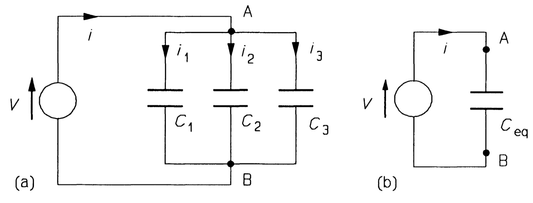
In figure the voltage is the same across each capacitance and KCL produces
\[i=i_1 +i_2+i_3\]Then using the \(i-v\) relation for capacitances, \(i = C~dv/dt\), in equation yields
\[i= C_{1}\frac{dv}{dt}+C_{2}\frac{dv}{dt}+C_{3}\frac{dv}{dt}\] \[i= (C_{1}+C_{2}+C_{3})\frac{dv}{dt} = C_{eq}\frac{dv}{dt}\]and
\[C_{eq}=C_{1}+C_{2}+C_{3}\]it can be seen that capacitors in parallel add.
Capacitances in series
In figure KVL can be used to obtain \(v = v_1 + v_2 + v_3\) which, differentiated with respect to \(t\), gives
\[\frac{dv}{dt}=\frac{dv_{1}}{dt}+\frac{dv_{2}}{dt}+\frac{dv_{3}}{dt}\]Now the current is the same in all three capacitors, thus
\[i=C_{1}\frac{dv_{1}}{dt}=C_{2}\frac{dv_{2}}{dt}=C_{3}\frac{dv_{3}}{dt}\]so that \(\frac{dv_{1}}{dt}= \frac{i}{C_{1}}, \frac{dv_{2}}{dt}= \frac{i}{C_{2}}\), etc., and equation becomes
\[\frac{dv_{1}}{dt}= \frac{i}{C_{1}}+\frac{i}{C_{2}}+\frac{i}{C_{3}} = \frac{i}{C_{eq}}\]where
\[\frac{1}{C_{eq}}=\frac{1}{C_{1}}+\frac{1}{C_{2}}+\frac{1}{C_{3}} \]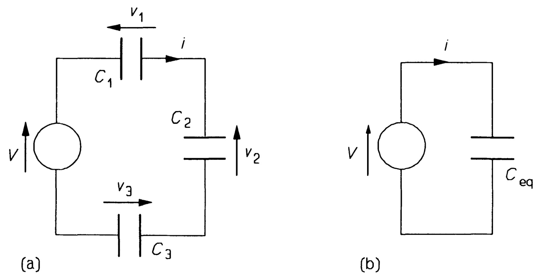
Circuit theorems and transformations
Many theorems and transformations (all derived from Kirchhoff's laws) can be used to assist with circuit analysis
Thevenin's theorem
Thevenin's theorem states
Any two-terminal, linear network of sources and resistances may be replaced by a single voltage source in series with a resistance. The voltage source has a value equal to the open-circuit voltage appearing at the terminals of the network. The resistance value is the resistance that would be measured at the network's terminals when all the sources have been replaced by their internal resistances.
Thevenin's equivalent circuit is shown in figure. To replace complex networks by such a simple equivalent circuit can be highly convenient. For example let us find the Thevenin equivalent of the two-terminal network of figure. There are three steps in essence. First, is to determine the voltage across AB. That is just the voltage across the 4 \(\Omega\) resistance, which may be found by the voltage divider rule as the resistances are in series with the voltage source:
\[V_{AB} = V_{4\Omega} = 4 \times \frac{3}{6} = 2~V\]This is the open-circuit voltage across \(AB\), and consequently the source voltage, \(V_T\), in the Thevenin equivalent circuit.
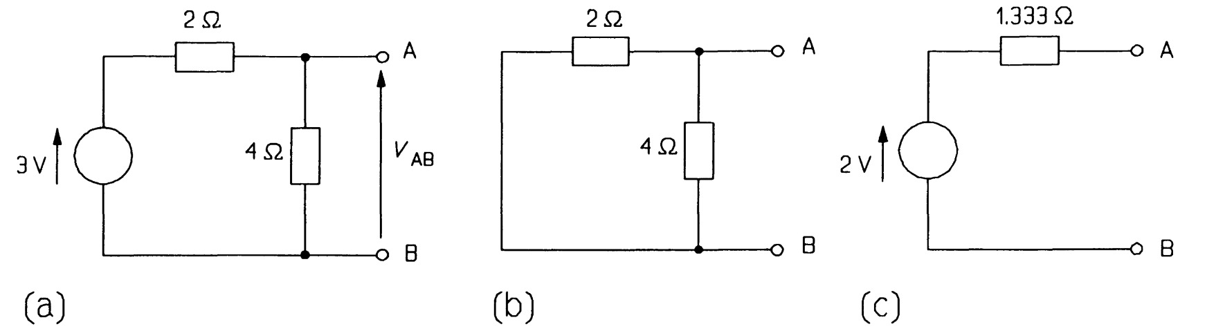
Secondly, the voltage source must be replaced by its internal resistance. As the voltage source is ideal and thus has zero internal resistance by definition, all this means is replace the voltage source by a short circuit. The circuit then becomes that of figure (b) simply two resistances in parallel when looked at from \(AB\). So, thirdly, we combine them by the product-over-sum rule:
\[R_{T} = \frac{2 \times 4}{2+4} = 1.333~\Omega \]Hence the Thevenin equivalent of the network in figure (c). It is important to realise that the circuits of figures are equivalent only for measurements of current and voltage made at terminals \(A\) and \(B\), and nowhere else.
Norton's theorem
Norton's theorem is a useful complement to Thevenin's:
Any two-terminal, linear network of sources and resistances may be replaced by a single current source in parallel with a resistance. The value of the current source is the current flowing between the terminals of the network when they are short-circuited. The value of the resistance is the resistance measured at the terminals of the network when all sources have been replaced by their internal resistances.
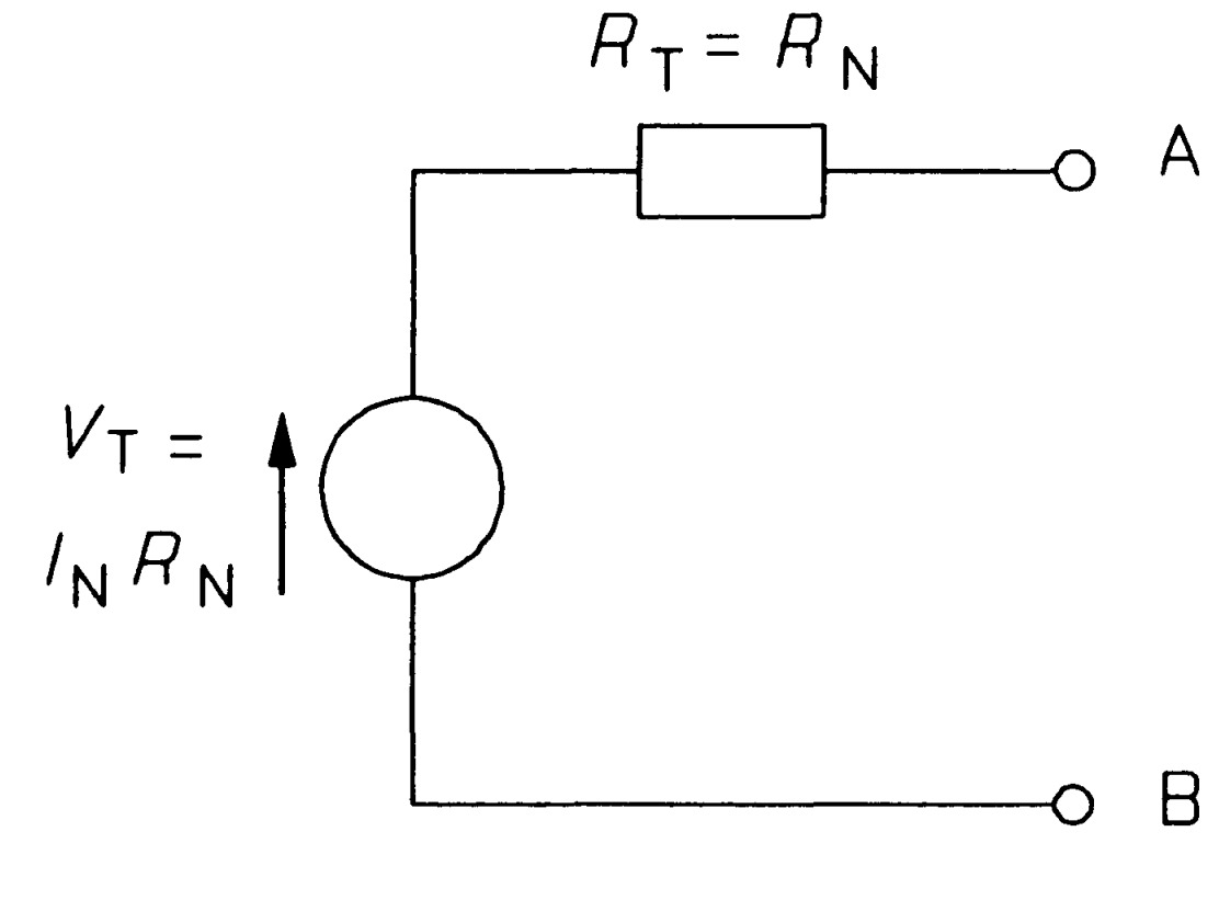
Norton's equivalent circuit is shown in figure.
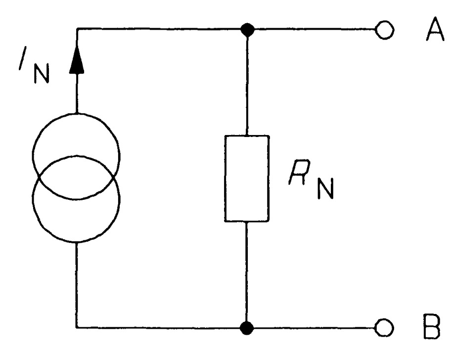
Any two-terminal network of sources and resistances may be replaced by this AB. Since Thevenin's theorem applies to any two-terminal network, it must apply to Norton's equivalent circuit too. The Thevenin equivalent of Norton's circuit can be derived as follows: In figure the open-circuit voltage is that across \(R_{N}\), which must be \(I_{N}R_{N}\) since all the current from the source flows through it. Therefore
\[V_{T}=I_{N}R_{N}\]The next step is to replace the source by its internal resistance - infinity for an ideal current source by definition - which amounts to open-circuiting an ideal current source. On doing this we are left with RN alone connected across AB, so the Thevenin resistance is identical to the Norton resistance:
\[R_{T}=R_{N}\]Figure shows the transformation, which requires only the calculation of \(V_T=I_{N}R_{N}\), the open-circuit voltage of Norton's equivalent circuit. We must decide for ourselves whether we use the Norton or the Thevenin form of equivalent circuit. As a general rule one should use the Norton circuit to combine parallel sources and the Thevenin circuit to combine series sources.
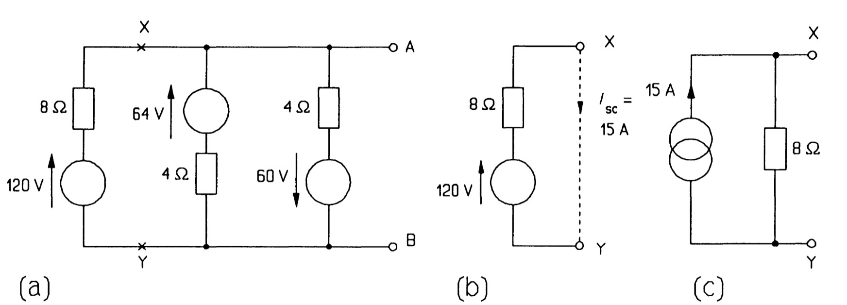
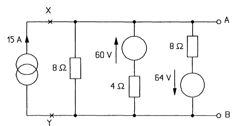
For example, consider the three generators in parallel in figure. We proceed by cutting the circuit at \(XY\) and looking at the source on the left by itself, as in figure. This source is in Thevenin form and must be transformed to the Norton form to enable us to add the parallel sources. The Norton source current is the current flowing through a short circuit across \(XY\), which is \(120/8 = 15 A\), by Ohm's law; and the Norton resistance is equal to the Thevenin resistance, 8 \(\Omega\). So the Norton form of the 120 V source is as in figure. Note that the current arrow has the same direction as the voltage arrow of the original source. It is a good idea if in doubt to check this by examining which way current would flow through the short-circuited terminals. Having transformed the source we can re-attach it to the network at \(XY\) as in figure. The next voltage source is then transformed (it makes no difference which way round the voltage source and its series resistance are placed), and finally the one nearest to \(AB\). In the latter case the Norton equivalent must have its current arrow pointing down, like the voltage source it replaced. Figure shows the circuit at this stage.
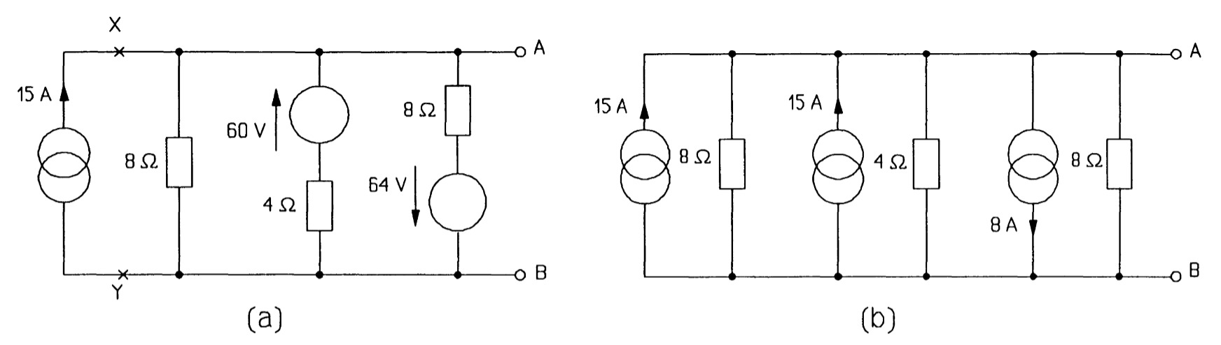
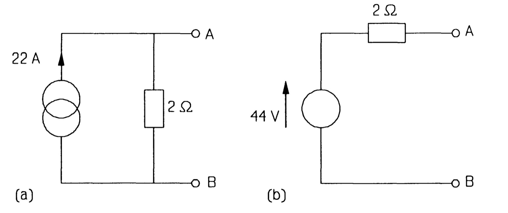
The three parallel current sources can now be added algebraically to give a single source of \(15 + 15- 8 = 22 A\). The third current source's value is subtracted from the other two as its direction is down and not up. Then the three parallel resistances in figure are combined to give a single 2\(\Omega\) resistance (by adding the reciprocals and taking the reciprocal of the result), giving the Norton circuit of figure . Finally the Norton circuit is turned into the Thevenin circuit of figure, using \(V_T = I_NR_N\).
The superposition theorem
Sometimes it is helpful to consider separately the effects of sources on a particular part of the circuit; the superposition theorem lets us do that. It states
The current in any branch of a circuit, or the voltage at any node, may be found by the algebraic addition of the currents or voltages produced by each source separately. When the effect of one source is being considered, the other sources are replaced by their internal resistances.
Superposition is most useful when the sources are alternating sources of differing frequency, or a combination of direct and alternating sources, but we can illustrate the use of superposition with direct sources alone.
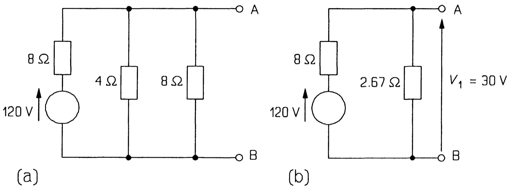
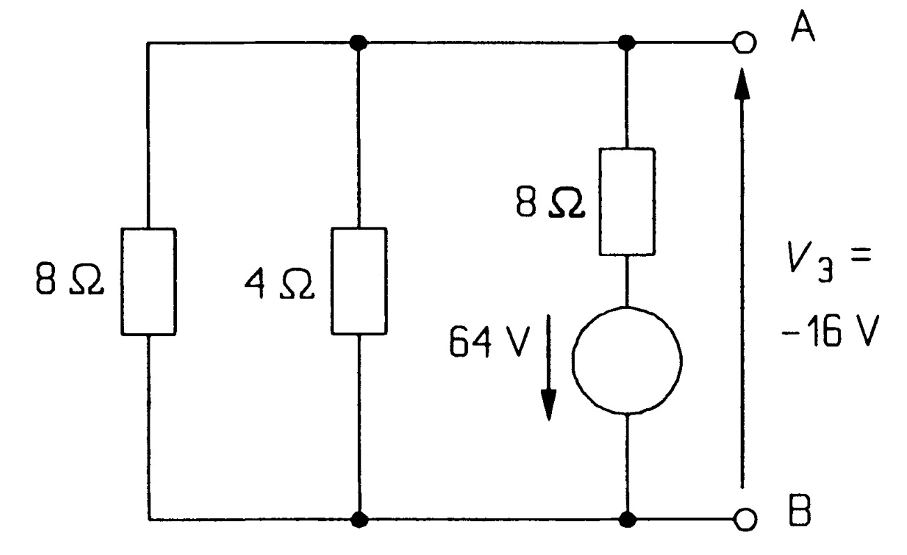
Consider the circuit of figure once more in which we wish to find V AB using superposition. For this we must add the voltages produced across AB by each source in turn.
Summing:
\[V_{AB} = V_{1}+V_{2}+V_{3}\]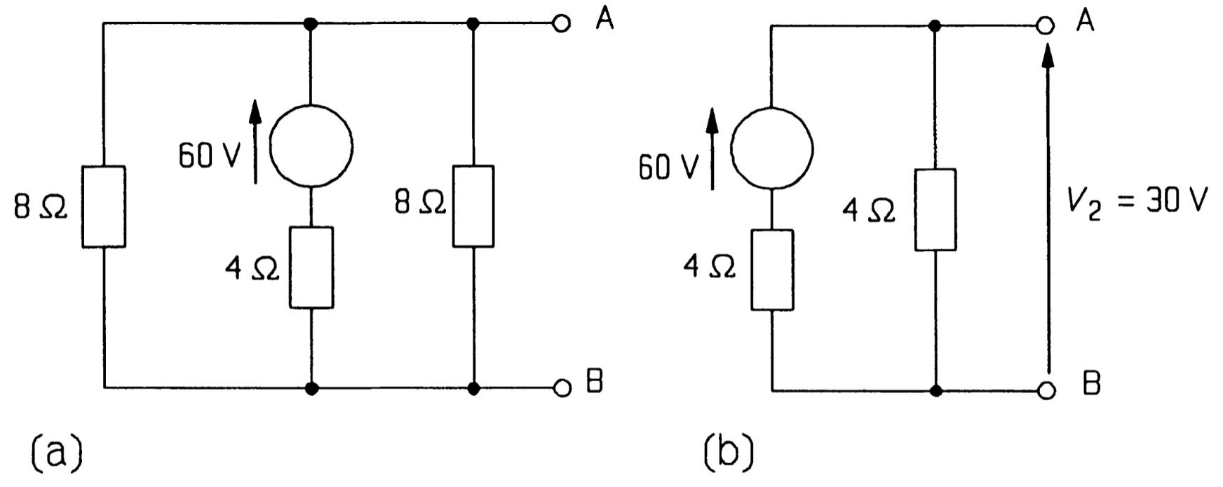
The result agrees with that found by source transformations. In general the superposition theorem is not very useful for solving problems in this mahner as it is too lengthy when three or more sources are present.
The star-delta transformation
Networks containing components that are neither in series nor in parallel are frequently encountered; the star-delta transformation enables us to change the form of networks like these so that they may be more readily analysed. In figure is shown a 3-terminal network in delta form, while the star form is in figure.
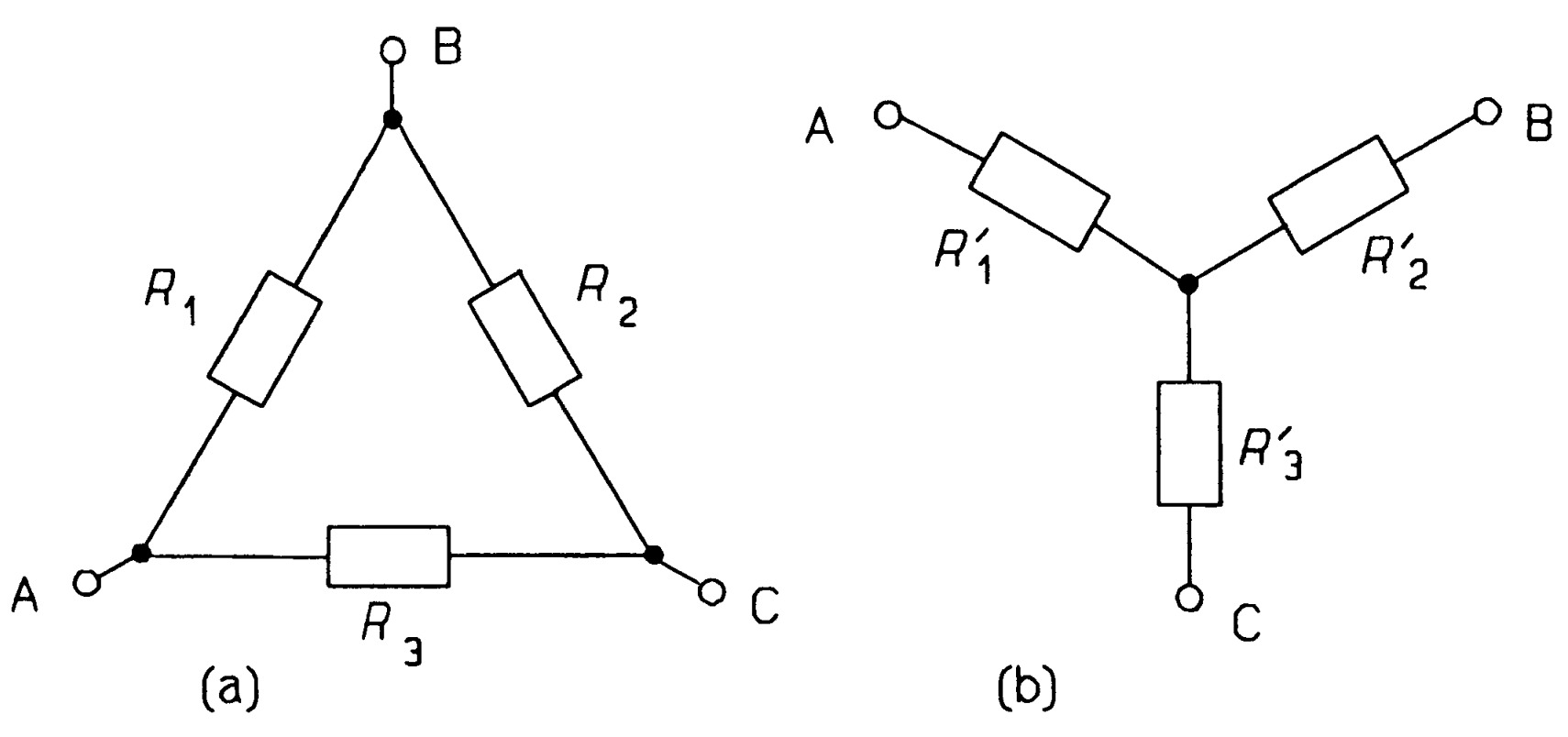
In North America, principally, this transformation is called the \(T-\pi\) (Tee-Pi), or \(Y-\pi\) (Wye-Pi) since it can be drawn in these shapes too, as in figure. Although this form looks like a four-terminal network, terminals \(3\) and \(4\) are common. The networks are equivalent if we can find the values of one set of resistances in terms of those of the other. \(Pi~(\pi)\) and Tee (\(T\)) equivialent circuits. The third and fourth terminals are common.
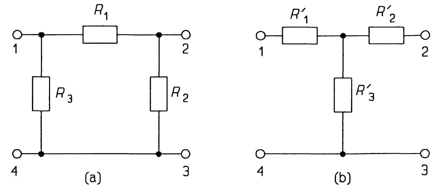
To calculate the resistance of the network of figure between terminals \(1\) and \(4\), we see that it comprises \(R_3\) in parallel with the series resistances, \(R_1\) and \(R_2\). In symbols, \(R_3 || (R_1 + R_2)\), to give (by the product-over-sum rule)
\[\frac{R_3(R_1 + R_2)}{R_1 + R_2 + R_3} =\frac{R_3(R_1 + R_2)}{\sum~R} ~~~~~~~~~~~~~~~~(1)\]where \(\sum~R = R_1 + R_2 + R_3\). Looking into the same terminals in second figure we see the resistance is \(R'_1 + R'_3\) and this must be the same for both networks, that is
\[R'_1 + R'_3= \frac{R_3(R_1 + R_2)}{\sum~R}~~~~~~~~~~~~~~~~(2)\]Then the resistance between terminals 2 and 3 is
\[R'_2 + R'_3= \frac{R_3(R_1 + R_3)}{\sum~R}~~~~~~~~~~~~~~~~(3)\]and looking into terminals 1 and 2 the final equation is obtained
\[R'_1 + R'_2= \frac{R_1(R_2 + R_3)}{\sum~R}~~~~~~~~~~~~~~~~(4)\]Subtracting equations \(2-3\) to find \(R'_1 +R'_2\) :
\[R'_1 - R'_2= \frac{R_1R_3-R_1R_2}{\sum~R}~~~~~~~~~~~~~~~~(5)\]Adding equations 4 and 5 yields
\[2R'_1 = \frac{2R_1R_3}{\sum~R}~~~~~~~~~~~~~~~~(6)\]or
\[R'_1 = \frac{R_1R_3}{\sum~R}~~~~~~~~~~~~~~~~(7)\]Solving for \(R'_2\) and \(R'_3\) similarly leads to
\[R'_2 = \frac{R_1R_2}{\sum~R}~~~~~~~~~~~~~~~~(8)\]and
\[R'_3 = \frac{R_2R_3}{\sum~R}~~~~~~~~~~~~~~~~(9)\]These transformations are easier to remember than it may appear. For instance the formula for \(R'_1\) (the resistance attached to terminal! of the star form) is just the product of the two resistances attached to terminal 1 of the delta form, divided by the sum of all three resistances. \(R'_2\) and \(R'_3\) are found the same way.
It is left as an exercise to show that the reverse transformation from star to delta requires
\[G_1 = \frac{G'_1G'_2}{\sum~G'}~~~~~ G_2 = \frac{G'_2G'_3}{\sum~G'}~~~~~G_3 = \frac{G'_1G'_3}{\sum~G'}~~~~~~~~~~~~~~~~(10)\]Remembering this is also easy, since each formula involves just the conductances between a pair of terminals. The letters DSR are a helpful mnemonic - Delta to Star: use Resistances - the reverse transformation must then employ conductances.
Power and energy
Electric power is given by
\[p =vi~~~~~~~~~~~~~~~~(1)\]p is in watts (W) if v is in volts and i in amperes. This enables us to find the power sent out by a voltage or current source, or the power dissipated in a resistance.
Energy is given by
\[E = \int p~dt = \int vi~dt ~~~~~~~~~~~~~~~~(2)\]Generally, \(v\) and \(i\) are the quantities usually measured, calculated or otherwise known, so equation 2 is more useful than the converse relation \(p = dE/dt\). From equations 1 and 2 we can derive others: for example, the voltage across a resistance is \(iR\) by Ohm's law, so the power dissipated in it as heat will be
\[p = vi = i^2R ~~~~~~~~~~~~~~~~(3)\]Only resistances dissipate energy, while inductances and capacitances store it: equation 2 can be used to find the amount stored. In the case of a capacitance, \(C\), the current is given by \(i = C~dv/dt\), therefore
\[E=\int vi~dt = \int vC\frac{dv}{dt}~dt = \int^{V}_{0}Cv~dv = \frac{1}{2}CV^{2}~~~~~~~~~~~~~~~~(4)\] \[E= \frac{1}{2}CV^{2}~~~~~~~~~~~~~~~~(5)\]In a like manner we may deduce that energy stored by an inductance of L henries carrying a current, I amps, is
\[E=\frac{1}{2}LI^{2}~~~~~~~~~~~~~~~~(6)\]The maximum power transfer theorem
Maximum power is transferred to a load resistance connected between two terminals of a network when the load resistance is equal to the resistance of the network measured between the same two terminals, the sources of the network being replaced by their internal resistances.
The proof is as follows. Any two-terminal network can be reduced to a single voltage source in series with a resistance (Thevenin's theorem) as in figure.
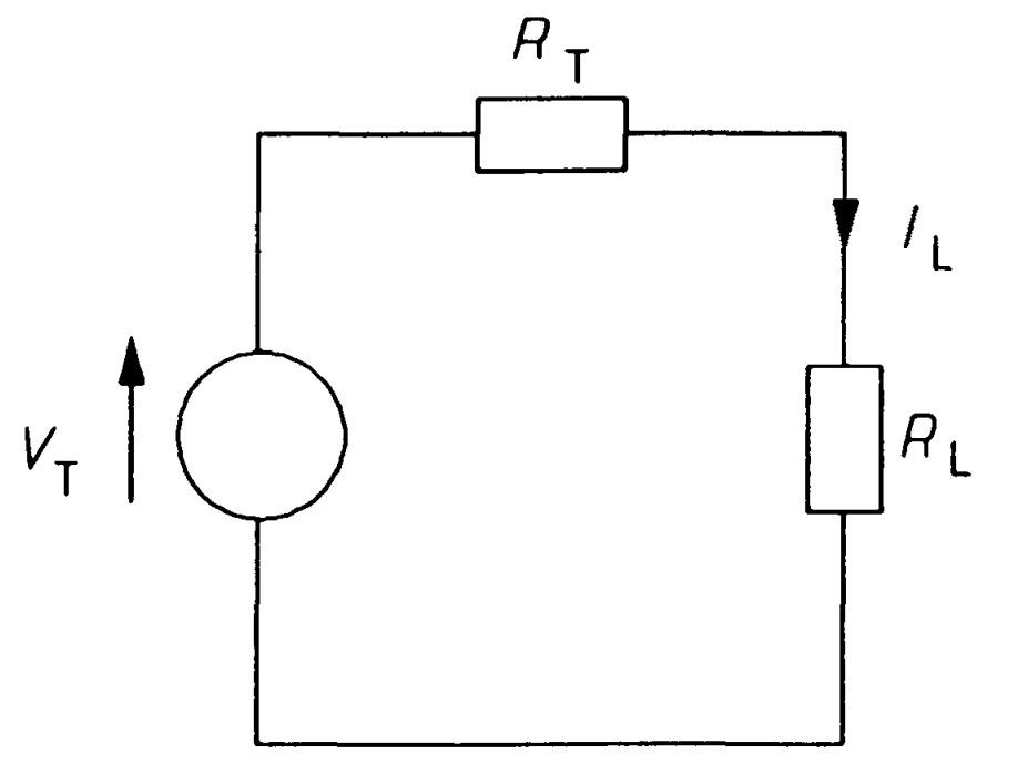
If a resistance, \(R_L\) is attached across AB, the current through it by Ohm's law is
\[I_L=\frac{V_T}{(R_T+R_L)}~~~~~~~~~~~~~~~~(1)\]The power developed in the load is
\[P_L=I_L^2R_L=\left[\frac{V_T}{(R_T+R_L)}\right]^2R_L~~~~~~~~~~~~~~~~(2)\]Differentiating with respect to \(R_L\) and equating to zero for turning points in \(P_L\)
\[\frac{dP_L}{dR_L}=\left[\frac{V_T^2(R_T+R_L)^2-2V_T^2(R_T+R_L)R_L}{(R_T+R_L)^4}\right]=0~~~~~~~~~~~~~~~~(3)\] \[V_T^2(R_T+R_L)^2=2V_T^2(R_T+R_L)R_L~~~~~~~~~~~~~~~~(4)\] \[R_T +R_L = 2R_L~~~~~~~~~~~~~~~~(5) \]that is
\[R_T = R_L~~~~~~~~~~~~~~~~(6)\]It is left as an exercise to check that this condition leads to maximum power in the load by deciding if \(\frac{d^2P_L}{dR_L^2}\) is negative. The maximum power transfer theorem reduces to
Maximum power is transferred from a resistive network when the load resistance is equal to the Thevenin resistance of the network.
When \(R_T = R_L\), the current through the load must be \(V_T/2R_L\), so the maximum power developed will be \(\frac{I^2_{max}}{R_L}\), or
\[P_{max}=\left(\frac{V^2_TR_L}{2R^2_L}\right)=\left(\frac{V^2_T}{4R_L}\right) ~~~~~~~~~~~~~~~~(7)\]It is worthwhile to emphasise here that transferring maximum power to a load will not result in maximum efficiency of power use, since at least half of the power consumed by the whole system must be lost in the source network. Maximum power transfer is most desirable when the source is weak, such as the signal from a radio or TV aerial, as it enables one to maximise the signal-to-noise ratio.
Mesh analysis and nodal analysis
Until now, we have used Kirchhoff's laws only in very simple circuits, for a good reason: without systematic use, they rapidly generate a large number of unknown quantities (though also equations by which they may be found). Mesh and nodal analyses are complementary ways of making systematic the application of Kirchhoff's laws to circuits, so that fewer errors are likely.
Mesh analysis.
Mesh analysis applies KVL systematically to a circuit and produces simultaneous equations that may be solved to give the mesh currents. A mesh is a loop in a circuit with no loops inside it. Consider the circuit of the figure, which represents a domestic 2-phase supply common in North America. It contains three meshes: ABCDA, ADEFA, and CEDC; the large loop ABCDEF A is not a mesh as it can be divided into smaller loops. The meshes have been numbered 1, 2, and 3. Meshes one and two represent low-voltage circuits for lighting and appliances such as vacuum cleaners, hair dryers, etc., while mesh three represents a two-phase circuit for supplying relatively large loads. The 0.1\( \Omega \) resistances represent the wiring resistance.
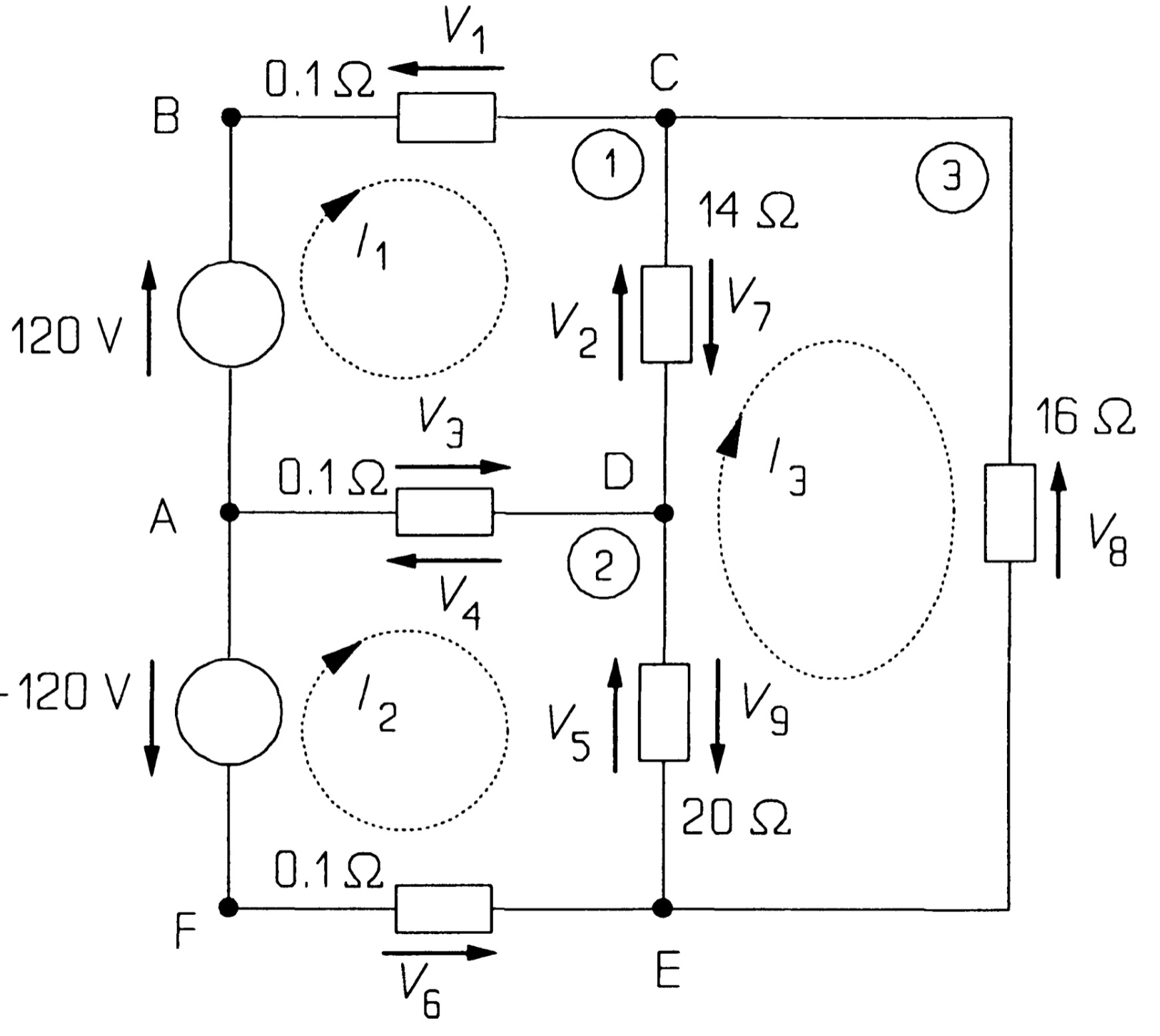
The first step in the analysis is to assign clockwise currents to each mesh: in this case, \( I_1 \), \( I_2 \), and \( I_3 \) to meshes 1, 2, and 3, respectively. The next step is to use KVL to find these currents. KVL around mesh 1 gives, with clockwise voltages taken as positive, anticlockwise negative:
\[ 120 - V_1 - V_2 - V_3 = 0 ~~~~~~~~~~~~~~~~~(1) \]\( V_1 \) is the voltage across the 0.1\(\Omega\) resistance, which by Ohm's law is 0.1\( I_1 \). \( V_2 \) is the voltage across the 14\( \Omega \) resistance, which is not 14\( I_1 \), since the 14\( \Omega \) resistance is shared between meshes, and the resultant current flow from C to D must be \( (I_1 - I_3) \). \( V_2 \) must therefore be 14\( (I_1 - I_3) \). \( V_3 \) is the voltage across the middle 0.1\( \Omega \) resistance (the common wire for the two phases), which is shared between meshes 1 and 2. \( V_3 \) must then be 0.1\( (I_1 - I_2) \) and equation 1 becomes
\[ 120-0.1I_1 -14(I_1 - I_3)-0.1(I_1 - I_2)=0 ~~~~~~~~~~~~~~~~~(2) \]or,
\[ 14.2I_1 - 0.1I_2 - 14I_3 = 120 ~~~~~~~~~~~~~~~~~(3) \]after rearranging terms.
The use of KVL in mesh 2 yields
\[ -(-120) - V_4 - V_5 - V_6 = 0 ~~~~~~~~~~~~~~~~~(4) \]The -120 V source points anticlockwise and is written -(-120) in equation 4 (if in doubt, reverse the arrow and the sign on this source, which leaves its value unchanged). \( V_4 \), the voltage across the middle 0.1 \( \Omega \) resistance, is 0.1 \( (I_2-I_1) \) by Ohm's law \( (V_4 = -V_3) \). \( V_5 \) is the voltage across the 20 \( \Omega \) resistance, and must be 20 \( (I_2-I_3) \) by Ohm's law, while \( V_6 \) is 0.1\( I_2 \), so that the equation becomes
\[ 120 - 0.1(I_2-I_1)-20(I_2-I_3)-0.1 I_3=0 ~~~~~~~~~~~~~~~~~(5) \]which rearranges to
\[ -0.1I_1, + 20.2I_2 - 20I_3 = 120 ~~~~~~~~~~~~~~~~~(6) \]Mesh 3 gives
\[V_7+V_8+V_9=0 ~~~~~~~~~~~~~~~~~(7)\]Again, the voltages are found by using Ohm's law:
\[ V_7 = 14(I_3 - I_1) ~~~~~~~~~~~~~~~~~(8)\], \[ V_8 = 16I_3 ~~~~~~~~~~~~~~~~~(9)\] and \[ V_9 = 20(I_3 -I_2) ~~~~~~~~~~~~~~~~~(10)\].Then, equation 7, after rearranging, is
\[ -14I_1 - 20I_2 + 50I_3 = 0 ~~~~~~~~~~~~~~~~~(11) \]Three meshes have produced three equations, numbered 12, 13 and 14:
\[14.2I_1 - 0.1I_2- 14I_3 = 120 ~~~~~~~~~~~~~~~~~(12)\] \[ -0.1I_1 + 20.2I_2- 20I_3 = 120~~~~~~~~~~~~~~~~~(13)\] \[ -14I_1 - 20I_2 + 50I_3 = 0 ~~~~~~~~~~~~~~~~~(14)\]Three meshes have produced three equations represented in matrix form:
\[ \begin{bmatrix} 14.2 & -0.1 & -14\\ -0.1 & 20.2 & -20\\ -14 & -20 & 50 \end{bmatrix} \begin{bmatrix} I_1 \\ I_2 \\ I_3 \end{bmatrix} = \begin{bmatrix} 120 \\ 120 \\ 0 \end{bmatrix} \]And there are three unknown mesh currents. The solution is \( I_1 = 23.1 \) A, \( I_2 = 20.6 \) A and \( I_3 = 14.7 \) A.
The currents through the 14\( \Omega \) and 20\( \Omega \) loads are \( I_1 - I_3 (= 8.4 A) \) and \( I_2 -I_3 (= 5.9 A) \), while the common wire carries a relatively small current \( I_1 -I_2 (= 2.5 A) \). The power consumed by the 14\( \Omega \) load is \( 14 \times 8.42 = 990 W\) , by the 20\( \Omega \) load is \( 20 \times 5.92 = 700 \) W, and the 16 \( \Omega \) load consumes \( 16 \times 14.72 = 3.5 kW\) .
Take note of the form of equations 12, 13, and 14: The first comes from applying KVL to mesh 1, so the coefficient of \( I_1 \) is opposite in sign to those of the other two currents. The second equation arises from applying KVL to mesh 2, so the coefficient of \( I_2 \) is positive and the rest negative. The third equation comes from mesh 3, so the coefficient of \( I_3 \) is positive, the others negative. If the unknown currents and voltages are assigned in the systematic way described, the signs of the current coefficients should always follow this pattern - check if they do not! With a little practice, the student will find it superfluous to put voltages across resistances and will be able to write down the current equations directly. Aided by a computer solution of simultaneous equations, an experienced student can solve a 7-mesh problem in two to three minutes and get it right the first time.
Nodal analysis
While mesh analysis employs KVL systematically, nodal analysis uses KCL to give a set of simultaneous equations from which all the nodal voltages may be derived. Voltages are assigned to each principal node of a network, principal nodes being points where three or more branches of a circuit join. Strictly, a node is the point at which two or more branches join, and a principal node is one where three or more branches join.
Consider the circuit of the figure. The (principal) nodes are A, C, D, and E, with node A being chosen as the reference node. (The reference node need not be at ground potential, nor at any particular place in the circuit: the choice is arbitrary.) Voltages are then assigned to the other nodes representing the potential differences between them and the reference node: these are \( V_1 \), \( V_2 \), and \( V_3 \) in the figure. We then apply KCL at nodes C, D, and E. At node C, taking the current out of the node to be positive, we see that
\[ I_1 + I_2 + I_3 = 0 ~~~~~~~~~~~~~~~~~(1)\]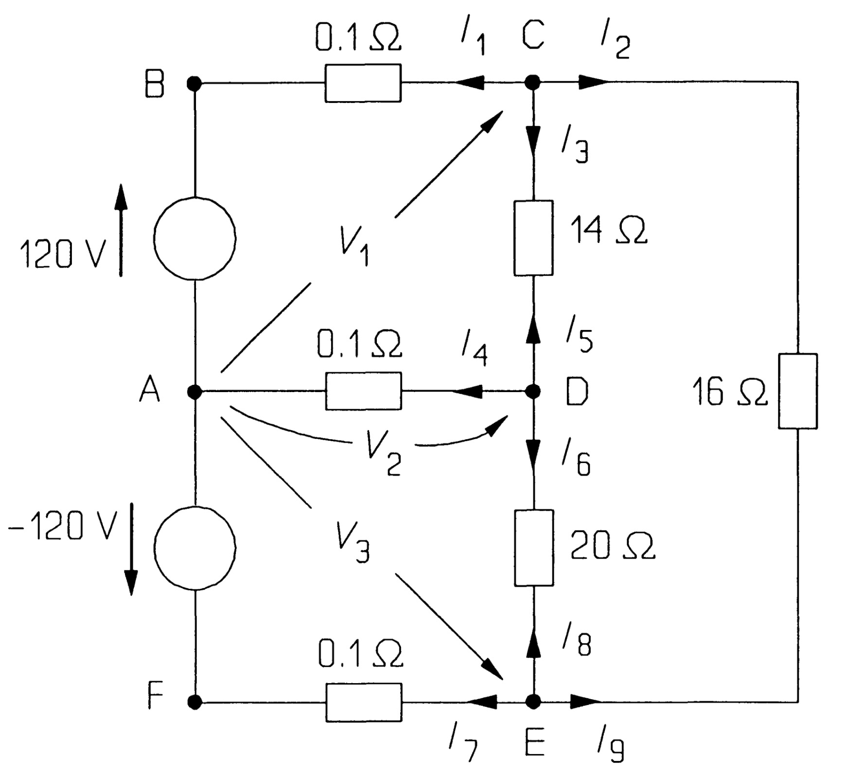
Now \( I_1 \) is the current through the uppermost 0.1\( \Omega \) resistance, which is given by Ohm's law as \( (V_1 - 120)/0.1 \) (make sure the sign is correct here!), since the voltage across the resistance is \( (V_1 - 120) \). Similarly, \( I_2 \) is \( (V_1 - V_3)/16 \) and \( I_3 \) is (V_1 - V_2)/l4. Equation 1 then becomes
\[ \frac{V_1 -120}{0.1}+\frac{V_1-V_3}{16}+\frac{V_1-V_2}{14}=0 ~~~~~~~~~~~~~~~~~(2) \]At node D,
\[ I_4 + I_5 + I_6 = 0 ~~~~~~~~~~~~~~~~~(3)\]Now \( I_4 = V_2 /0.1 \), as the middle 0.1\( \Omega \) resistance lies between the reference node A and node D, then \( I_5 = (V_2 - V_1)/14 \) (note that \( (I_5 = -I_3) \), but one should always give the currents at each node new identities, and work out afresh what they are) and \( ( I_6 = (V_2 - V_3)/20) \). Thus equation 3 is
\[ \frac{V_2}{0.1}+\frac{V_2-V_1}{14}+\frac{V_2-V_3}{20}=0 ~~~~~~~~~~~~~~~~~(4) \]Finally, at node E
\[ I_7 + I_8 + I_9 = 0 ~~~~~~~~~~~~~~~~~(5)\]where
\[ I_7 = (V_3 - (-120))/0.1 ~~~~~~~~~~~~~~~~~(6)\], \[ I_8 = (V_3 - V_2)/20 ~~~~~~~~~~~~~~~~~(7)\] and \[ I_9 = (V_3 - V_1)/16 ~~~~~~~~~~~~~~~~~(8)\].Substituting these values into equation 4 gives
\[ \frac{V_3 +120}{0.1}+\frac{V_3-V_2}{20}+\frac{V_3-V_1}{16}=0 ~~~~~~~~~~~~~~~~~(9) \]Rearranging equations 2, 4 and 9 produces the three simultaneous equations.
\[ 10.13V_1 - 0.071V_2 - 0.0625V_3 = 1200 ~~~~~~~~~~~~~~~~~(10)\] \[ -0.071 V_1 + 10.12V_2 - 0.05V_3 = 0 ~~~~~~~~~~~~~~~~~(11)\] \[ -0.0625V_1 - 0.05V_2 + 10.11 V_3 = -1200 ~~~~~~~~~~~~~~~~~(12)\]Three node equations are represented in matrix form:
\[ \begin{bmatrix} 10.13 & -0.071 & -0.0625\\ -0.071 & 10.12 & -0.05\\ -0.0625 & -0.05 & 10.11 \end{bmatrix} \begin{bmatrix} V_1 \\ V_2 \\ V_3 \end{bmatrix} = \begin{bmatrix} 1200 \\ 0 \\ 1200 \end{bmatrix} \]The solution to the equations is \( V_1 = 117.7 \) V, \( V_2 = 0.24 \) V and \( V_3 = -118 \) V.
The form of these equations is worth remarking: the first comes from using KCL at node C, where the voltage relative to node A is \( V_1 \), and the only positive coefficient is that of \( V_1 \). The same pattern is followed in the other two equations. Any mistakes in sign should soon be noticed and put right if the equations are written in this systematic way. The solution to the equations is \( V_1 = 117.7 \) V, \( V_2 = 0.24 \) V and \( V_3 = -118 \) V. The voltage across the 14 \( \Omega \) load is \( 117.7- 0.24 = 117.5 \) V, and the current through it is \( 117.7/14 = 8.4 \) A, as before. The voltage across the 20 \( \Omega \) resistance is \( 0.24- (-118) = 118.2\) V, so the current through it is \( 5.9 \) A, and finally, the voltage across the 16 \( \Omega \) resistance is \( 117.7 -(-118) = 235.7 \) V, and the current through it is \( 14.7 \) A. The solution is, as it must be, the same as that found by mesh analysis earlier.
Model Questions
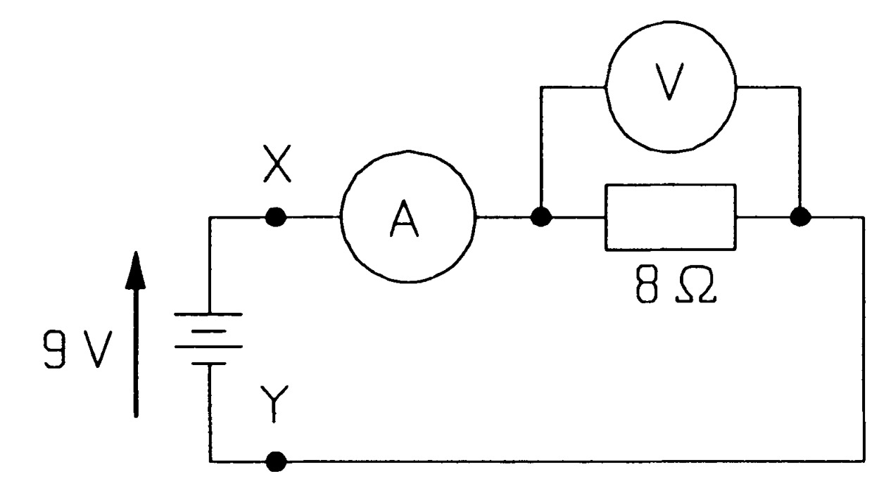
In the circuit of figure \(MQ1\) the battery has an internal resistance of 2 \(\Omega\), the ammeter one of 0.1 \(\Omega\) and the voltmeter one of 1 k\(\Omega\). What are the readings of the ammeter and voltmeter? What would the voltmeter read if it were to be reconnected across \(XY\)? \(Ans:[0.897~A, 7.117~V, 7.206~V]\)
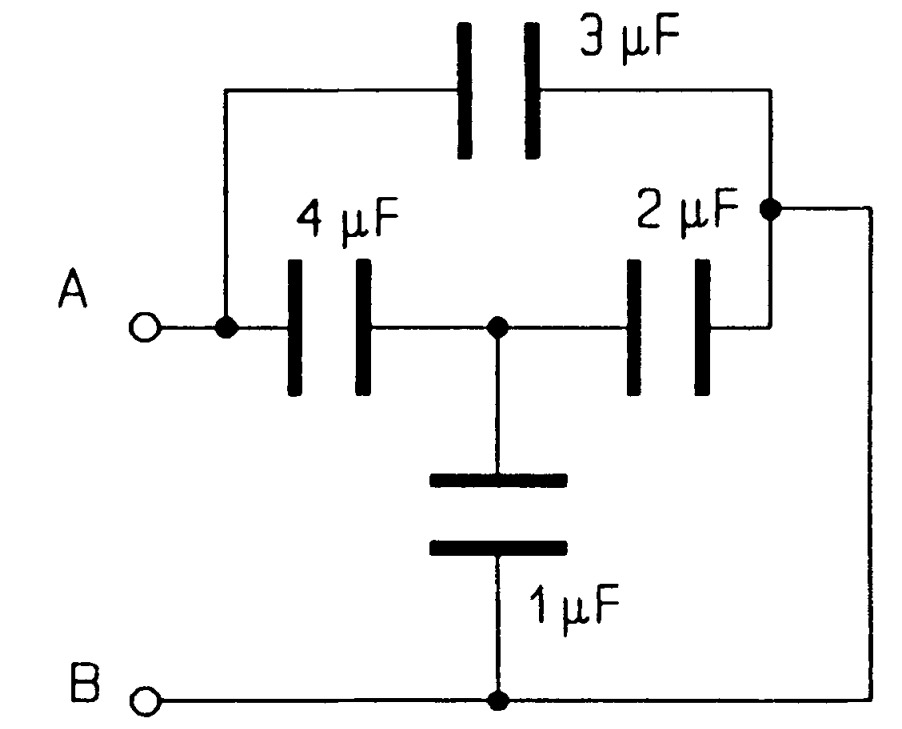
Find the equivalent capacitance between \(AB\) of the circuit of figure \(MQ2\). \(Ans:[1.86~\mu F]\)
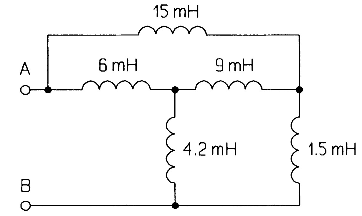
Find the equivalent inductance between \(AB\) of the circuit of figure \(MQ3\). \(Ans:[6~mH]\)
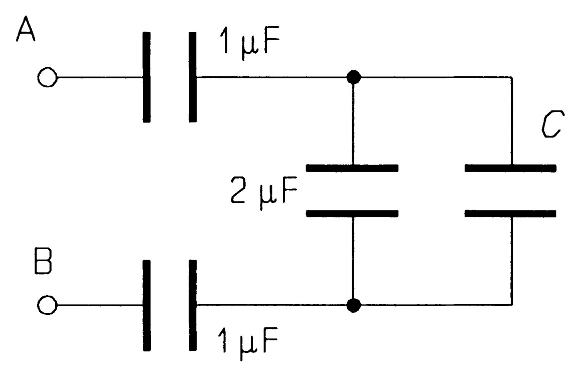
What must \(C\) be for the capacitance to be \(C\) between the terminals \(AB\) in figure \(MQ4\)? \(Ans:[0.414~\mu F]\)
You are given an ohmmeter of infinite accuracy and a large number of resistors of which all but one have exactly the same resistance. How can the odd resistor be found with just two measurements? \(Ans:[Hint:~connect~in~series/parallel~twice]\)
Use Kirchhoff's laws and the \(v-i\) relationship for inductors to show that inductors in series may be added like resistors for the equivalent inductance. Also show that inductors in parallel behave like resistors in parallel when their equivalent is required.
What is the resistance of the circuit formed by placing a resistance of \(6~\Omega\) along each edge of a cube and joining them at all eight corners? The resistance is measured between two corners at the opposite ends of the longest diagonal. \(Ans:[5~\Omega]\)
A capacitance of \(1~F\) is charged up to \(5~V\) and then is connected to an initially uncharged capacitance of \(2~F\) in series with a \(1~\Omega\) resistance. (a) What is the voltage across each capacitance after the connection is made? (b) What energy is stored in the circuit before and after the connection is made? (c) What energy is lost in the resistance? (d) Does the resistance affect the answer to (c)? (e) What happens to the energy if the resistance is zero? \(Ans:[(a) 1.67~V~and~-1.67~V~(b)~12.5~J~and~4.17~J~(c)~4.33~J~ (d)~No]\)
Show using a Thevenin equivalent circuit and a resistive load, that maximum power transfer does not result in maximum efficiency for energy transfer, and that for the latter the Thevenin resistance should be zero.
If all the energy stored in a \(32~pF\) capacitor charged to \(24~kV\) is transferred to an inductance of \(0.5~pH\), what is the current? (This is an exploding-wire experiment, but in practice the resistance slightly reduces the current.) \(Ans:[ 192~kA]\)
A superconducting magnet has been proposed for storing energy. If the current in the magnet is to be \(200~kA\) when the stored energy is \(5~GWhr\), what is its inductance? If the maximum allowable voltage across its terminals is \(5~kV\), what is the maximum rate of change of current? What is the minimum time needed to discharge all the stored energy? What is the average power delivered in this time? What is the maximum output power? How practical is this proposal? \(Ans:[900~H,~5.56~A/s,~10~hrs,~500~MW,~1~ GW]\)
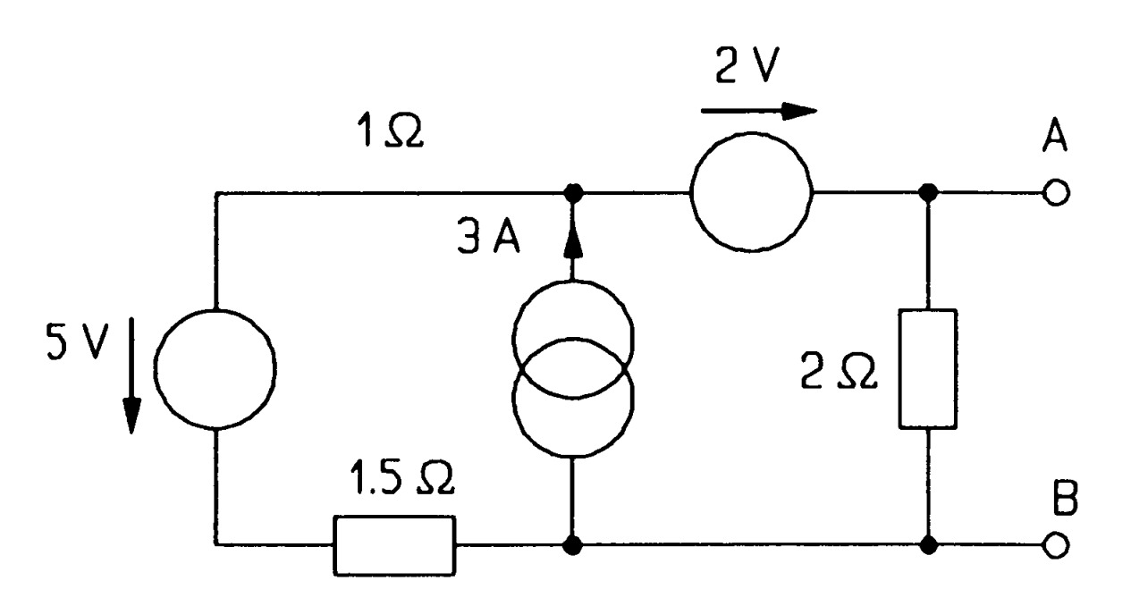
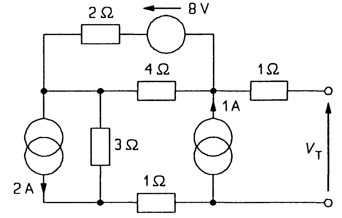
Find the Thevenin and the Norton equivalents of the circuit between \(AB\) in figure \(MQl2\). Find the maximum power transferable from these terminals. What power is consumed internally by the circuit when delivering maximum power (that is excluding the load) and unloaded? \(Ans:[V_T = 2~V, R_T = 1.11~\Omega, I_N = 1.8~A, 0.9~W, 6.9~W~and~12~W]\)
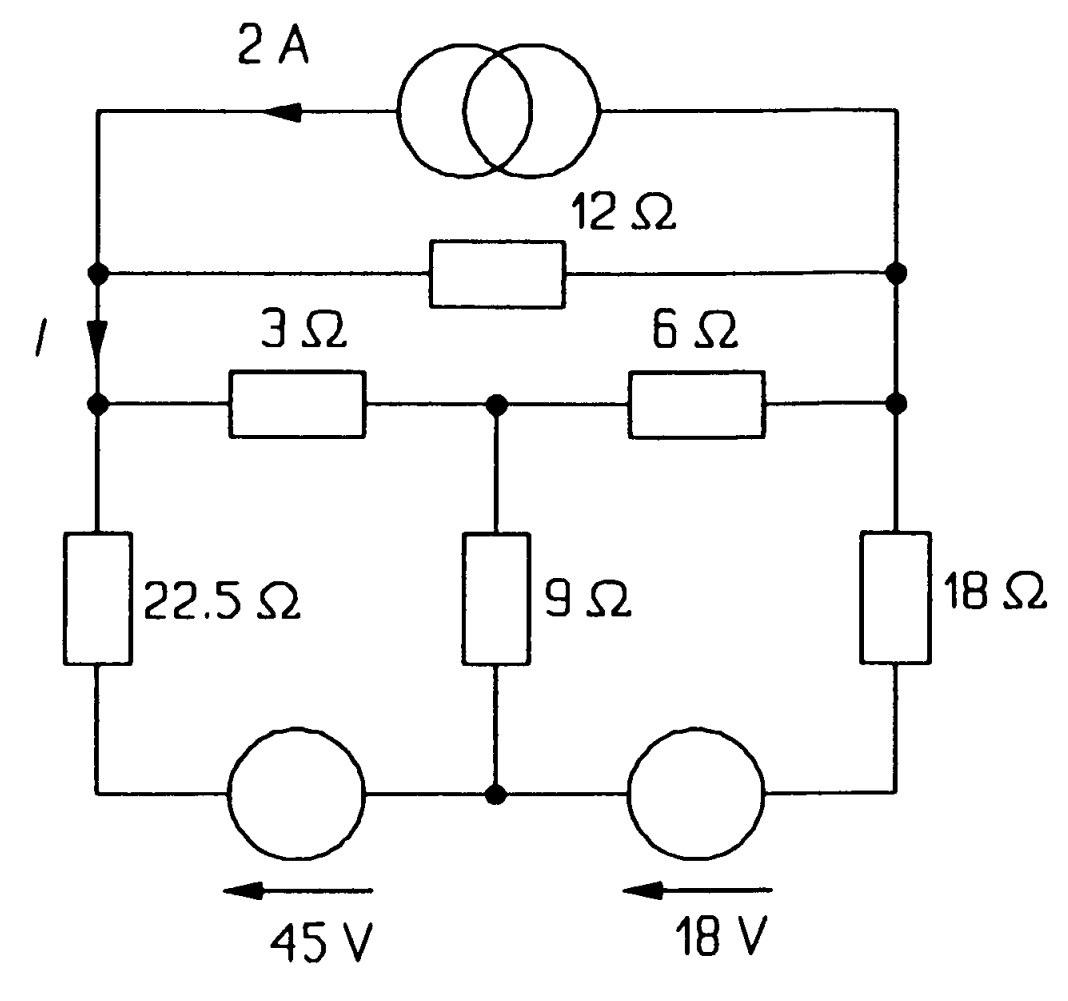
Use the star-delta transformation to find \(I\) in figure \(MQ13\). \(Ans:[I= 0.7~A]\)
Use mesh analysis to find the current from the \(18~V\) source in figure \(MQ13\). \(Ans:[0.815~A]\)
Use nodal analysis to find the voltage across the \(2~A\) source in figure \(MQ13\). \(Ans:[15.6~V]\)
Use Kirchhoff's laws and a full branch-current analysis to confirm the answers to problems \(13\), \(14\) and \(15\).
Use successively Norton's and Thevenin's theorems to find the voltage across \(AB\) in the ladder network of figure \(MQ17\). \(Ans:[4~V]\)
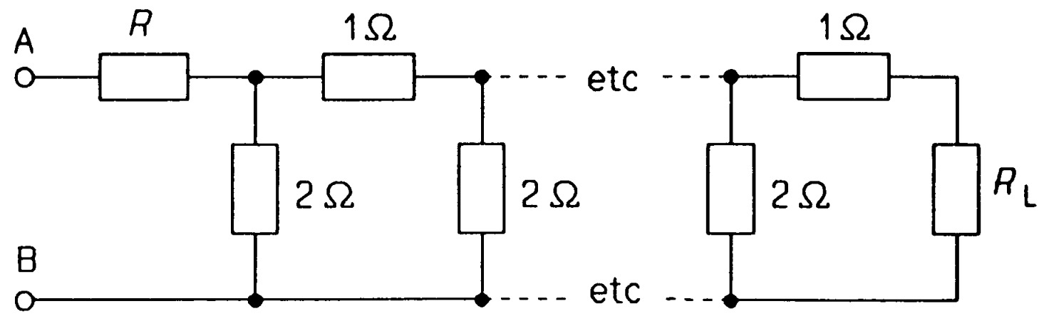
In the infinite network of figure \(MQ18\) what must \(R\) and \(R_L\) be for the resistance to be \(2~\Omega\) between terminals \(AB\)? \(Ans:[ 1~\Omega~and~any~resistance]\)
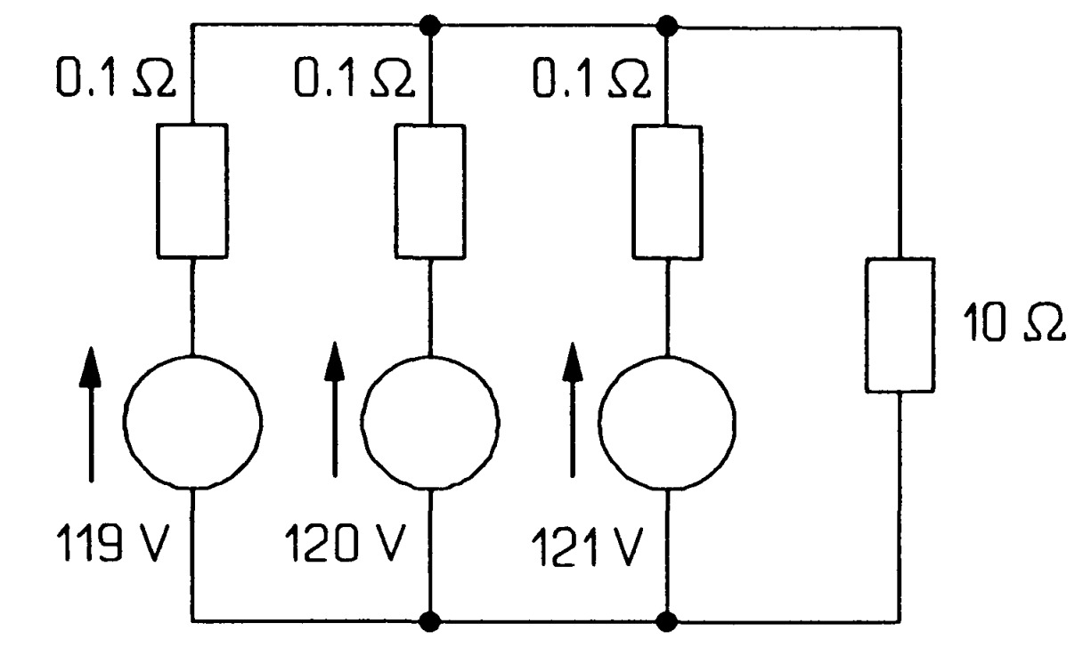
Find the power delivered by (a) the \(121 V\) (b) the \(120 V\) and (c) the \(119 V\) source in figure \(MQ19\). Repeat this problem when the source resistances are \(0.3 \Omega\) for the \(121 V\), \(0.2 \Omega\) for the \(120 V\) and \(0.1 \Omega\) for the \(119 V\) source. \(Ans:[(a)~1.692~kW~(b)~478~W~(c)~-716~W,~812~W, 607~ W~and~15~ W]\)
In the circuit of figure \(MQ20\), use the superposition principle to find \(V_T\) \(Ans:[ -6~V]\)
A capacitance of \(200~pF\) carries a current of \((2 + 3 sin 2t)~mA\). What is the voltage across it as a function of time, \(t\), if it was initially uncharged? \(Ans:[(10t - 7.5~cos2t)~V]\)
What is the energy consumed by a resistance of \(583 \Omega\) from time \(t = 0\) to \(t = 10~ms\) when the current through it is \(0.63~exp(-100t) A\)? What is the average power and \(r.m.s.\) current during this time? \(Ans:[1~J,~100~W,~0.414~A]\)
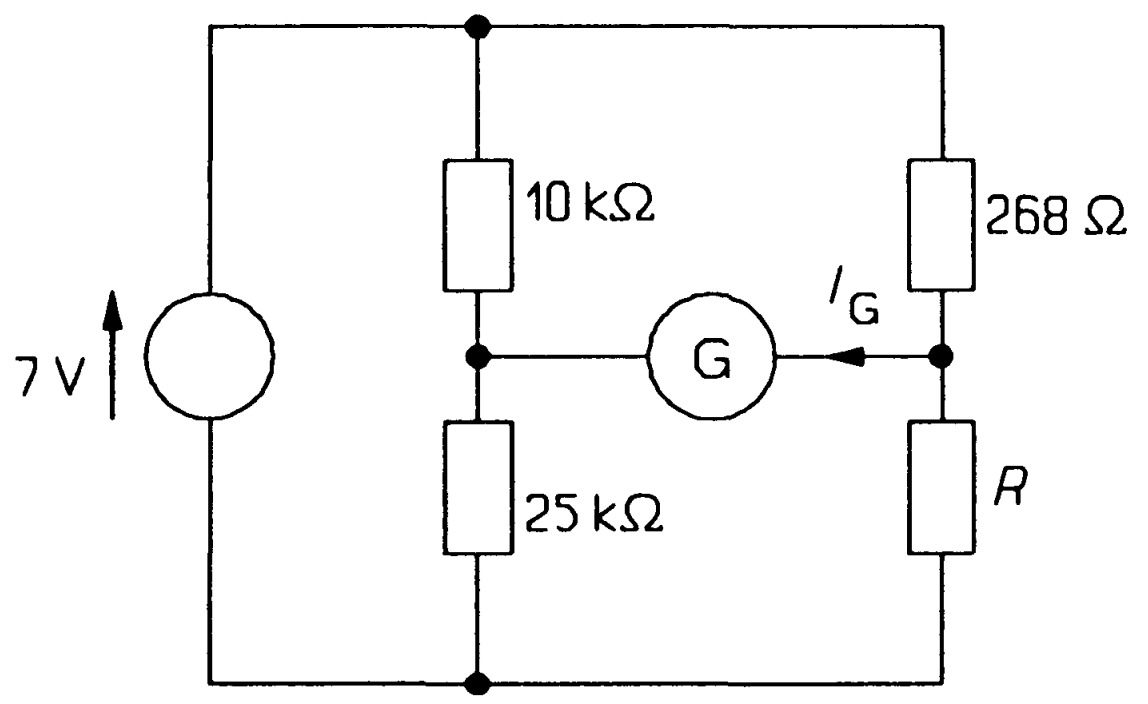
The bridge circuit of figure \(MQ23\) is used to measure the value of \(R\) using a resistanceless galvanometer to detect imbalance. If the galvanometer's minimum detection current, \(I_G\) , is \(0.1~pA\), what is the percentage error in \(R\)? \(Ans:[0.1\%]\)
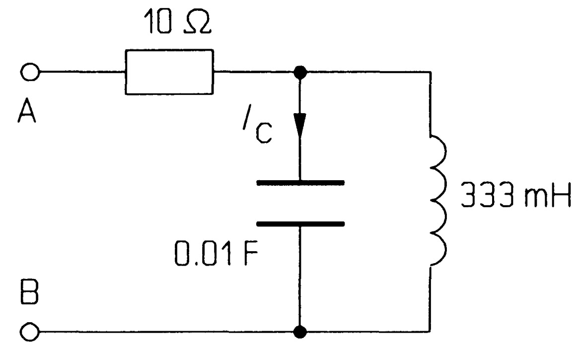
In the circuit of figure \(MQ24\) no energy is stored at time \(t= 0\). \(I_C\) is \(20t mA\) and starts from zero at \(t = 0\). What is the voltage across \(AB\) at \(t = 0.3 s\)? \(Ans:[0.42~V]\)
Show that the transformation from star form to delta form requires that the equations (\(10\) of the star-delta transformation) be satisfied.